Use the rticles package

When I first went about preparing my manuscript for publication, I was in minor despair. My intended journal provided style files for LaTeX, and I wasn’t sure how to apply those to my R Markdown document. I was worried I would have to hand-paste in the necessary header after generating a .tex file using knit. Doing this process one time isn’t so bad. However, if I went down this path, then every time I wanted to update the document, I would have to generate a new .tex file, and then re-do the cutting and pasting.

When I discovered the rticles package, I was saved. The rticles package provides easy to use R Markdown templates for a variety of journals. It also includes a nicely formatted template for arXiv. If you’re lucky enough to have your intended journal represented here, fantastic! If not, and you find an elegant solution, please tell me about it! You can also contribute your own template, or put out an open request for someone to develop the template you want.

If you cannot use the rticles package, there are almost certainly ways to avoid the manual process of pasting together documents in order to create your final manuscript. For example, you could generate a LaTeX fragment. A LaTeX fragment is a .tex file containing only LaTeX formatted writing, without any headers or \begin{document} tags, that can be then put into another document using \include{}. However, be warned that stitching together a LaTeX document from different files can sometimes be quite finicky.

Set convenient defaults

By convention, a R Markdown document begins with a setup code chunk.

I recommend adding some defaults to your setup chunk to make your life easier. Let’s start with knitr chunk options, which are set using knitr::opts_chunk$set(foo = bar). Note that any knitr options set in this global way will apply to not only the chunk that contains the line, but also all chunks below.

• cache = TRUE will save you time by caching all your results.
• warning = FALSE and message = FALSE avoids printing out pesky messages into your document.
• fig.height = 4 and fig.width = 3 set default sizes for your figures. I find fig.width especially useful as a global option, as you may need to constrain all your figure sizes at once if you change your document margins to fit a particular journal format. You can further scale figures using out.width = "50%", which means that the final output will be limited at maximum to be 50% of the width of the page.
• fig.align = "center" aligns your figures to the middle of the page.

Outside of chunk options, there are other useful things you can do in your setup chunk.

• set.seed(1234) to ensure your results don’t change across runs.
• options( knitr.kable.NA = '' ) controls how NA values are printed in tables.
• theme_set( theme_minimal() ) controls the default ggplot theme for any ggplot2 figures. The minimal theme simplifies plots such as removing the gray background and reducing the number of gridlines. The built-in themes for ggplot can be found here, and there are also a variety of themes available in other packages. For example, the ggthemes package has theme_tufte and theme_economist.

Warning. Although above I recommend caching results and turning off messages and warnings, it is good practice to periodically turn off these features. Clear your cache, turn on those messages and warnings, and make sure everything is working as intended! I have run into situations where my code was broken without me realizing it because it was running cached results, or because I was suppressing warnings and messages. You can clear your cache by going to the arrow next to Knit and selecting “Clear Knitr Cache.”

Restrain yourself

For me, one of the most powerful, and most dangerous, features of R Markdown is its flexibility. I have written documents that combine an unholy mix of LaTeX, R, markdown, CSS, and HTML. It is at times effective, but not always elegant or readable. The quick road to end up in such a mess is to use R Markdown, and then switch to, e.g., LaTeX to control some specific aspect of your document. For example, say you usually create lists using markdown formatting (- list item 1) but then sometimes use LaTeX formatting (\item) because you want to customize the list bullets in a way that is difficult in markdown. If you borrow from one place and another, it can get messy.

For your own sake, I recommend limiting yourself and try to stay in one language as much as possible, rather than mixing together typesetting from all of the formatting languages supported. If you are a LaTeX power user, and you are optimizing to write to a PDF, I strongly recommend sticking to LaTeX typesetting whenever possible. LaTex allows for easy global customizations that affect appearance across the document, such as removing section numbers, or changing the appearance of bullets in a list. If you write in markdown, you will instead have to use CSS if you want to change appearance from the defaults. Personally, I find CSS more unwieldy, but if you are a CSS master, go for it! Note that I do not know if all CSS formatting will appear in PDF documents.

As another example, you can write section headers using # or using \section{}. Let’s say you want to change if your section headers are numbered or not, and cross-reference sections automatically using \ref{}. These are features that are familiar to many LaTeX users, but are more difficult in CSS/markdown.

On the other hand, markdown has the advantage of simplicity. You may find there are fewer compilation errors because markdown forces you to follow the KISS principle: keep it simple, stupid! In some settings, it may be useful to not have the temptation of customization.

Manage citations

If you are only producing a PDF document, you can include citations via either R Markdown notation, @citation, or LaTeX notation, \cite{}. Again, changing the formatting of citations is generally more flexible with the LaTeX options.

To use natbib, import the package in your R Markdown header, as below. Then, cite as normal in the document using \citep and \citet and include the bibliography where you wish using \bibliography{refs}.

title: "My Super Awesome Paper"
author: "Me"
date: "`r format(Sys.time(), '%B %d, %Y')`"
output: 
  pdf_document:
    keep_tex: TRUE
header-includes:
   - \usepackage{natbib}
   - \bibliographystyle{abbrvnat}
   - \setcitestyle{authoryear, open={((},close={)}}

Bonus: the call to Sys.time() automatically sets the date to the current date.

Side note. If you decided to use R Markdown citations, and you want to submit to arXiv, this strategy can present a small problem. arXiv does not take .bib files, and instead only accepts .bbl files. Knitting your document will not generate a .bbl file if you use R Markdown citations. Also, you can’t easily create your own .bbl file, because in the generated .tex files, the citations will already be rendered (i.e. @Smith2000 in the .Rmd file will be Smith (2002) in the .tex file, not \cite{Smith2000}). There is however a way to get around this. In LaTeX, create an empty .tex document with \nocite{*} (see below) to generate citations for all your references, and then compile that outside of R. Then upload the .bbl file along with your compiled .tex from your real markdown document.

\documentclass{article}

\begin{document}

\nocite{*} % generate bibtex entries for all references
\bibliography{refs} 

\end{document}

Compiling this document produces a .bbl file, which you can then upload to arXiv. Note that this will generate bibtex items for all items in your .bib file, so you will need to restrict that file to only references you actually cite. Obviously, the process I have outlined for creating a .bbl file is annoying, and you can avoid it by using LaTeX citations instead of R Markdown citations!

Make beautiful tables effortlessly

If you are creating a table by printing out a dataframe, you can create a beautiful table with ease. Starting with the built-in knitr::kable() options:

• Setting booktabs = TRUE produces nice formatting, and results in publication-ready tables.
• You can specify the number of significant digits to print using digits.
• The position parameter allows you to specify LaTeX-style positions. See this post for a brief introduction to LaTeX position options. Note that LaTeX is very opinionated on table locations, so often it will override your requested position.

In addition, the kableExtra package provides a variety of nifty table styling options. Here, I only use it to center the table, but it also creates striped tables and other pretty formatting.

library(knitr)
library(palmerpenguins)
library(tidyverse)

# change NA's to print as dashed lines
options(knitr.kable.NA = '-')

# print table
knitr::kable( penguins[1:5, 1:5], digits = 3,
              booktabs = TRUE, format = 'latex',
              position = "h!", caption = "Penguins!" ) %>%
  kableExtra::kable_styling( position = "center" )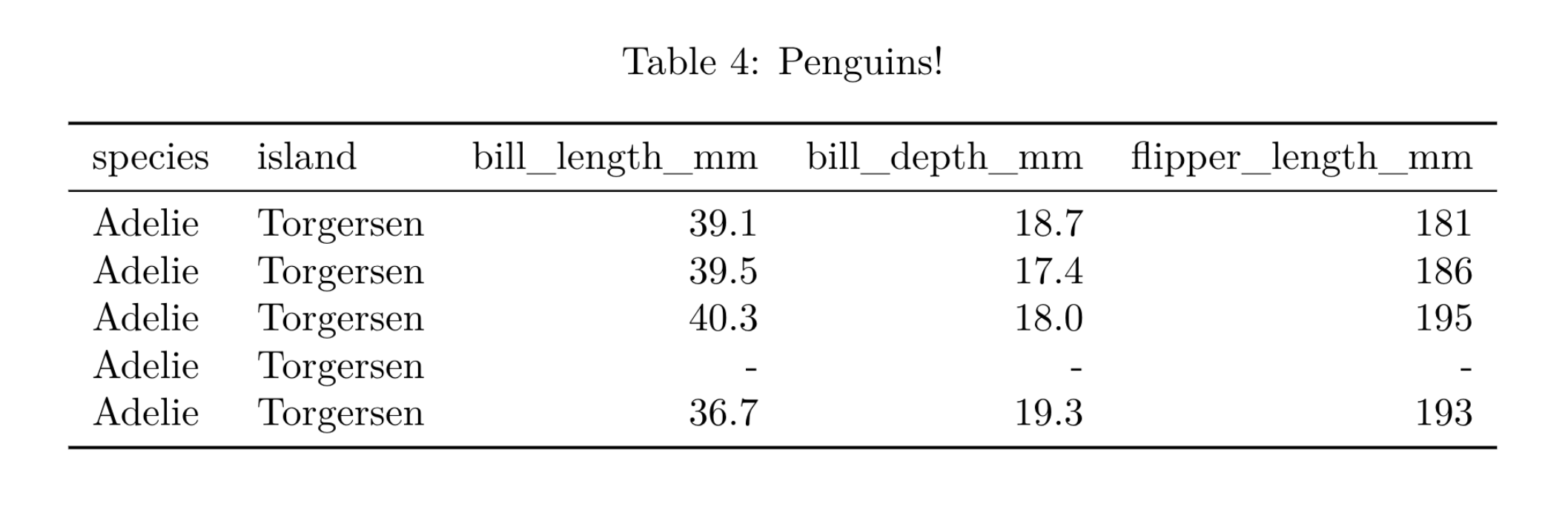

Compare this to a default table.

options(knitr.kable.NA = NA)
knitr::kable( penguins[1:5, 1:5], caption = "Penguins!" )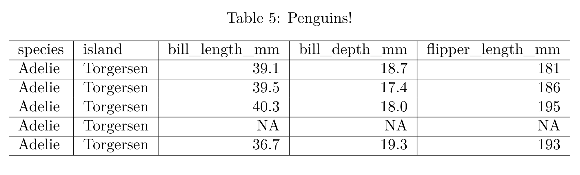

If you want to refer to a table, you can refer to it using the name of the code chunk. If penguinTable is the name of the code chunk, you can refer to it using \ref{tab:chunk-name}, such as “Table \ref{tab:penguinTable} shows penguin data.” R Markdown automatically adds the tab: notation. Similarly, if it were instead a figure in code chunk penguinFigure, you would refer to “Figure \ref{fig:penguinFigure}. Note: using \ref{} to only works if the figure/table has a caption; without a caption, LaTeX will not generate a number for the float.

Both for easy referencing and for good style, you should only have one output (either a table or figure) per code chunk; you should not include multiple figures or tables in the same chunk, although R Markdown does allow you to do so. One exception to this guideline is if you want to automatically generate multiple tables or figures using a for loop. However, this strategy does make your life complicated. To put outputs in a loop, you need to force the output to be raw R Markdown using the results = 'asis' chunk option.

You may also need to use results = 'asis' for outputs from certain packages like stargazer. Essentially, stargazer has already produced all the necessary formatting, so if you don’t call results = 'asis' then knitr tries to add additional formatting, and the table does not render properly. For more information about raw R Markdown, see the R Markdown Cookbook.

Finally, for pdf documents, if you want to insert a table by hand, you can use the standard \begin{table} LaTex approach.

Some tips on debugging

When a R Markdown document fails to compile because of a LaTeX error, the offending document line is given to you, but it references the line in the LaTeX document, not the R Markdown document. The rticles package defaults to saving out the generated .tex files, so you can open up the .tex file to trace back the error. If you are not using the rticles package, you can add keep_tex = TRUE to your header to make sure the .tex file is saved (as shown in the header example above). You can also play with the LaTeX file directly if you find it is easier for debugging: open up your .tex file in your favorite LaTeX compiler and re-compile the document to see the errors. Then, trace back to what changes you need to make in the R Markdown document.

I used the rticles package to create a template, dumped in my manuscript…and of course found my document would not compile, but not due to a LaTeX error! The error message I got was not very useful, so I tried stripping down my document, removing pieces to try and get it to compile. Depending on your confidence, you can take either a bottom-up or top-down approach for compilation errors. For a bottom-up approach, you can begin with a minimal document that actually compiles, and add on until you hit the error. For a top-down approach, you can remove one thing at a time to see which one produced the error. For example, for a bottom-up approach, you can remove all customization (loading packages, special table formatting, etc.). Alternatively, if it is annoying to remove certain customizations (such as not wanting to re-write all your tables), you can start with a single section in the document that compiles, and comment out the rest of the document. Then, add back sections of the document until you hit the error.

In my case, I discovered that there was a clash between the R Markdown template and the table options I was using from kableExtra. Unfortunately, this clash meant that if I wanted my nicely-formatted tables, I wasn’t able to print them automatically. To keep the code for reference, I added include = FALSE, eval = FALSE in the chunk options so that I could keep it in the document, but the chunk would not run. Then, I generated the LaTeX output by hand. To hand-generate LaTeX output, paste the code that generates the table and run it in the console, and it will output the appropriate LaTeX. If you run the code in the R Markdown document instead of in the console, it will automatically render the table instead of outputting the raw LaTeX output. Finally,copy the LaTeX output from the console and paste it into the document. The final document would look as below.

```{r penguinTable3, include = FALSE, eval = FALSE}
knitr::kable( penguins[1:5, 1:5], caption = "Penguins!", format = "latex" )
```

\begin{table}

\caption{Penguins!}
\centering
\begin{tabular}[t]{l|l|r|r|r}
\hline
species & island & bill\_length\_mm & bill\_depth\_mm & flipper\_length\_mm\\
\hline
Adelie & Torgersen & 39.1 & 18.7 & 181\\
\hline
Adelie & Torgersen & 39.5 & 17.4 & 186\\
\hline
Adelie & Torgersen & 40.3 & 18.0 & 195\\
\hline
Adelie & Torgersen & NA & NA & NA\\
\hline
Adelie & Torgersen & 36.7 & 19.3 & 193\\
\hline
\end{tabular}
\end{table}

This step is only a minor inconvenience, but it does mean I need to be careful to re-generate my tables if I change any code! I have no idea how common a clash like this is, and it did not occur with the other template I tried.

A smaller issue that I ran into: R happily takes either single or double quotes in most settings. However, some of the templates don’t play so nicely with single quotes. In R Markdown documents, it is good practice to consistently use double quotes in R code.

Make re-usable R Markdown chunks

One of the best parts of R Markdown is its flexibility. You can turn R Markdown into a paper, blog post, package vignette, or package readme file. In all likelihood, there will be some overlap in content between these different documents. For your own sake, and for the sake of reproducibility, you may want to write a snippet once, and re-use it across different documents. Check out this nice post about how to reuse R Markdown snippets.

Name your chunks

When the R Markdown is compiling, it references where it is in the document by saying it is working on something like unnamed-chunk-3. It is good practice, although not required, to name your code chunks for easier reference. The name of the code chunk is also used as the name of any figures that are generated and saved. Knitting a document called foo generates a folder called foo_files with a subfolder called figure-latex. This folder contains all the generated figures based on the chunk name, so if you name your chunk plot-bar you will end up with plot-bar.pdf instead of unnamed-chunk-12-1.pdf. Having named chunks is also convenient so you know where your code is slow–it’s easier to diagnose if your render is hanging on the calculate-baz chunk rather than unnamed-chunk-14. In the end, however, you can happily avoid naming chunks if you prefer. Also note that knitr will reject duplicated chunk names.

Use your ORCID

It is recommended for authors to use their ORCID, which is a unique personal identifier, so that John Smith publishing ecology papers in Wisconsin is disambiguated from John Smith publishing geometry papers in Oslo. The LaTeX orcidlink package provides an easy way to include your ORCID. However, I found it was not included in my Rstudio LaTeX distribution, so I couldn’t just add \usepackage{orcidlink} to my document header. An easy fix is to go to the package github site and download just orcid.sty. When I placed that file in the same directory as my document, \usepackage{orcidlink} worked, and I could add a link to my ORCID page by adding \orcidlink{4444-4444-4444-4444} after my name.

Conclusion

Despite some quirks, I recommend writing manuscripts in R Markdown, especially if your paper directly incorporates either code itself, or a lot of code output. For journals that have no rticles template available, or for manuscripts with little direct output, it may not be worth the extra effort. However, for my situation, the difficulties of getting the document into publication-ready format were well worth the effort over the boring and mistake-prone process of updating tables and figures by hand each time I changed a tiny aspect of my analysis.