Plotting distributions of site-level impact estimates (or other collections of noisily estimated things)
by Luke MiratrixDo you ever want to visualize the distribution of effects across sites in a multi-site evaluation (or meta analysis)? For example, consider a multisite trial with 30 sites, where each site is effectively a small randomized experiment. A researcher might fit a multilevel model with a random effect for the impact in each site, allowing for cross-site impact variation, and then want to plot these results. How should they do this?
Visualizing the distribution of impact estimates turns out to be tricky business. In this post we look at some of the trickiness, and talk through one solution people (e.g., Bloom et al. (2017)) have used to get out from under it.
This post is built on some work that recently got accepted at JEBS, “Improving the Estimation of Site-Specific Effects and their Distribution in Multisite Trials” (Lee et al. (2024), ArXiV draft (here)). In this work, colleagues and I looked at different combinations of strategies including so-called triple-goal estimation and using nonparameteric Bayesian methods to identify best practices for this sort of estimation. We also identified different aspects of a context that make estimation more or less tractable. This post is a distillation of some lessons learned, and a presentation of a simple fix that gets most of the bang for only a few bucks.
Ok, let’s look at four options for plotting a distribution of site-level impact estimates:
- Plot the raw estimates
- Plot the Empirical Bayes estimates we get from a multilevel model
- Plot these same Empirical Bayes estimates, but rescaled by our estimated amount of impact variation
- Plot the density curve implied by the fitted multilevel model
Each of these methods have some plusses and minues. Let’s walk through what they all actually are, and then we will compare them to each other on a few toy datasets.
Raw estimates are too loose
A multisite trial is just a bunch of simple randomized trials, and we can analyze each one independently. Consider \(J\) sites, with students nested in the sites. For each student we have, for student \(i\) in site \(j\), \(Z_{ij} = 1\) if they are treated and \(Z_{ij} = 0\) if not. For each site we could ignore the other sites and estimate the site-level impact \(\beta_j\) as the simple difference in means of treated and control students in that site: \[ \hat{\beta}_j = \overline{Y}_{1j} - \overline{Y}_{0j}, \] where \(\overline{Y}_{zj}\) is the mean of all students in site \(j\) with \(Z_{ij} = z\).
We then could simply plot the distribution of the \(\hat{\beta}_j\), but this turns out to be a bad idea (unless the sites are very large). The reason is our \(\hat{\beta}_j\) are over-dispersed (too spread out); consider, for example, that even if all the true \(\beta_j\) were the same, the \(\hat{\beta}_j\) would still be scattered around due to estimation error. Even worse, if we have a few very small sites, those sites will have very noisy estimates, making our plot look like it has large tails of extreme site-level average impacts.
To formalize the problem, model our estimated \(\hat{\beta}_j\) as \[ \hat{\beta}_j = \beta_j + r_j ,\] where \(\beta_j\) is the true site-level average impact and \(r_j\) is the error in measuring this impact. Now, assuming independence between the size of the true impact and the size of the standard error across sites, we have \[ Var(\hat{\beta}_j) = Var(\beta_j)+Var(r_j) = \tau^2 + SE_j^2 .\] The spread (or variance) of the distribution of effect estimates is a combination of variation in the true effects of the interventions (\(Var(\beta_j)\)) plus independent variation in estimation error (\(Var(r_j)\)). Accordingly, the distribution of effect estimates would be wider (and sometimes much wider) than the distribution of true effects (for more details, see Bloom et al. (2017) and Hedges and Pigott (2001)).
Empirical Bayes estimates are too tight.
To fix this, we might turn to multilevel modeling. With multilevel modeling, we first estimate the amount of treatment variation we have, and then we use that measure to shrink our raw individual site estimates towards the overall average impact. This is Empirical Bayes (EB) estimation.
For example, for student \(i\) in site \(j\) we might fit the Random Intercept, Random Coefficient (RIRC) model of \[ Y_{ij} = \alpha_j + \beta_j Z_{ij} + \epsilon_{ij}, \] with \((\alpha_j, \beta_j) \sim N( (\mu, \beta), \Sigma )\) as the random intercept and random treatment impact for site \(j\), and with \(\Sigma\) being a \(2 \times 2\) variance-covariance matrix of these random effects.
These days we might instead fit the Fixed Intercept, Random Coefficient (FIRC) model (Bloom et al. 2017), which is as above except we let the \(\alpha_j\) be fixed effects and only put a random effects distribution on the \(\beta_j\), with \(\beta_j \sim N( \beta, \tau^2 )\), where \(\tau\) is the cross-site impact variation. For more on the FIRC model, and estimating the amount of impact variation across sites, see our post, “Fitting the FIRC Model, and estimating variation in intervention impact across sites, in R”.
Regardless, we first fit one of these models to our data, getting \(\hat{\beta}\), the estimate of the average impact across sites, and \(\hat{\tau}^2\), the estimated amount of cross-site impact variation.
Empirical Bayes is then a second step procedure that “shrinks” the raw \(\hat{\beta}_j\) estimates towards the overall estimated ATE \(\hat{\beta}\), with the amount of shrinkage depending on the precision of the original \(\hat{\beta}_j\) and the amount of estimated variation \(\hat{\tau}\). Roughly speaking, the Empirical Bayes estimate \(\tilde{\beta}_j\) are \[ \tilde{\beta}_j = p_j \hat{\beta}_j + (1-p_j) \hat{\beta} , \] where \(p_j\) is the weight placed on the raw site-specific estimate \(\hat{\beta}_j\) vs. the overall average estimate \(\hat{\beta}\). You can think of \(p_j\) as approximately being \[ p_j \propto \frac{ \tau^2 }{ \tau_2 + SE^2_j }, \] where \(SE_j\) is the standard error for \(\hat{\beta}_j\). If a site is big, we have a good measure of the impact in that site, so the standard error will be low, sending the \(p_j\) towards 1, meaning we mostly tend towards the individual site estimate. If the site is small, the \(p_j\) will tend towards 0, meaning we mostly tend towards the overall cross-site average estimate. If we estimate that there is not much cross-site impact variation, then all the \(p_j\) will tend towards 0, which will cause greater shrinkage.
This differential shrinkage is a very nice thing about Empirical Bayes estimates. Because the smaller sites, with corresponding greater levels of uncertainty, get shrunk more than larger sites, Empirical Bayes prevents the small sites from having the largest estimated impacts just due to their greater levels of error.
Unfortunately, raw Empirical Bayes estimates tend to be over-shrunk, meaning that overall our \(\tilde{\beta}_j\) will be pulled in too far towards the overall mean. If we then plot the \(\tilde{\beta}_j\), we will get a histogram that is generally too narrow. For further discussion of this, you can see the section about “adjusted” E-B impact estimates (see formula 33) of Bloom et al. (2017). This general point can also be found on page 88 of Raudenbush and Bryk (2002) (a seminal text on MLM).
The reason we get over-shrinkage is that the shrinking is designed to give us the best prediction for each individual site. Say ten of our sites in some larger trial all have about the same estimated, somewhat large, \(\hat{\beta}_j\) and are all about the same size. For each individual site, we would shrink in towards the overall ATE. But if we step back and look at the full collection of ten estimates, we would recognize that a few of these sites really might have large impacts, but we just don’t know which ones. We thus shrink them all as the shrinkage is not looking globally, but is instead acting locally. That being said, by shrinking the estimates, we may help combat “the winner’s curse” (Simpson 2022) or “promising trials bias” (Sims et al. 2022).
Rescaling gets it just right?
For individual sites, Empirical Bayes is the best choice, but if we are looking at the distribution of impacts, can we offset this “overall too small” problem?
We can at least try, because our multilevel model directly provides a handy direct estimate, \(\hat{\tau}\), of how much cross site impact variation there is. We can use \(\hat{\tau}\) to rescale our \(\tilde{\beta}_j\) so they have the same standard deviation as we think they should, based on our multilevel model. This rescaling, called “Constrained Bayes” (Ghosh 1992), is the approach discussed and used in Bloom et al. (2017).
More specifically, we calculate adjusted EB impact estimates of \[ \check{\beta}_j = \hat{\beta} + \frac{\tau}{SD(\tilde{\beta}_j)} \left( \tilde{\beta}_j - \hat{\beta} \right) . \] Rescaling before visualization seems like a fine idea—in particular, the distribution of the final estimates will have the exact variation as we estimated with our model, and so our histogram will have the right spread, even if not the right shape—but it still has some real problems. In particular, the shrinkage, the estimate of \(\tau\), and the rescaling all depend on the original model, with the normality assumption, being correct. If the true distribution of impacts is not normal, this process will distort the estimates towards normal, which can be somewhat deceptive. See Lee et al. (2024) for further discussion. This point is worth pausing on: in general, we often can be quite cavalier about Normality. OLS, for example, is quite robust to violations of normality, especially if we use robust standard errors, and the central limit theorem often saves us, as it does here with respect to being able to assume \(\hat{\beta}_j \sim N( \beta_j, SE_j)\) to close approximation. There is no central limit theorem helping with the distribution of the \(\beta_j\), however, and the Normality assumption ends up doing a lot of work. If it is wrong, we can get some pretty bad results, as we will see below.
And finally, if we truly believe the normality assumption, we perhaps should commit fully to the model and plot the normal curve \(N( \hat{\beta}, \hat{\tau}^2 )\) implied by the estimated \(\hat{\beta}\) and \(\hat{\tau}\) instead of using any of this Empirical Bayes business. Unfortunately, the parametric curve turns out to be overly rigid: the flexibility of the Empirical Bayes estimates does allow some of the true shape to come through and the direct use of the Normal curve allows none of it.
To make all this blather more concrete, let’s see how these four methods work on a sample dataset.
A test drive of the methods
To illustrate how each of the four approaches of raw estimates work, and to provide code for implementing them, I generated synthetic data mimicking a multisite experiment with 100 sites, and substantial variation in the number of students in each site (size ranges uniformly from 20 to 80 students).
The standard deviation of the control side outcomes, across all sites, is 1, putting us in effect size units.
The true mean impact of the data generating process is \(ATE = 0.2\), and the true standard deviation of the \(\beta_j\) distribution is 0.2.
Our final data, of 5,162 rows, one row per student, consists of three variables: site id (sid), treatment assignment (Z), and observed outcome (Yobs).
It is worth noting that we have an additional complication: are we trying to estimate the true distribution for the sample we have (a finite-sample inference problem) or the true distribution of some superpopulation where the sites in our sample came from? In particular, for the specific dataset we generated, the true mean and standard deviation of the \(100\) site-level impacts is 0.198 and 0.185; these are not exactly the same as the parameters in our data generating process. But these are parameters in their own right: they are not estimates, but descriptives of the data we have. In general, we view all the estimation approaches discussed as targeting finite-sample quantities (this is also what we do in our paper); in the following, we report both finite- and super-population estimands so you can see how they differ.
Raw estimates
To get raw estimates for each site, we fit an interacted fixed effect model, allowing individual estimates for each site, and then pull out the coefficients for the interactions. The “0 +” tells R to not have a grand intercept, and the “sid:Z” not an overall average effect; the combination gives a fixed intercept and impact estimate for each site.
J = length( unique( dat$sid ) )
Mols = lm( Yobs ~ 0 + sid + sid:Z, data=dat )
beta_raw = coef(Mols)[(J+1):(2*J)]
mean( beta_raw )
## [1] 0.204sd( beta_raw )## [1] 0.335Our estimated variation in impacts, sd( beta_raw ), is too high, as anticipated—this is the over-dispersion discussed above.
Empirical Bayes estimates
We can fit a FIRC model easily in R by taking advantage of a different blog post that shows how to use a package from the CARES lab, blkvar, to fit a FIRC model:
library( blkvar )
ests = estimate_ATE_FIRC( Yobs, Z, sid, data=dat )
ests
## Cross-site FIRC analysis (REML)
## Grand ATE: 0.192 (0.0337)
## Cross-site SD: 0.209 (0.0152)
## deviance = NA, p=NAThe top line shows the overall average treatment effect estimate and standard error for that estimate. We next see the estimated cross-site impact variation, also with a nominal standard error (not to be particularly trusted, it turns out). The estimate cross-site impact variation of 0.21 is about right. The above blog post gives details and original R code to show what is going on under the hood.
We get the Empirical Bayes estimates with a call to get_EB_estimates():
betas = get_EB_estimates( ests )
sd( betas$beta_hat )
## [1] 0.129Note how the standard deviation of our final EB estimates is substantially less than the estimated amount of variation; this is the over-shrinkage.
Rescaled EB estimates
To rescale our EB estimates, we first pull the estimated average impact and estimated cross-site impact variation from the originally fit model with:
ATE = ests$ATE_hat
tau = ests$tau_hat
We then rescale as so:
sd_EB_est = sd(betas$beta_hat)
betas$beta_scale = ATE + (tau/sd_EB_est) * (betas$beta_hat - ATE)
Our rescaled estimates have a standard deviation of 0.21, exactly what our multilevel model estimated.
Density estimates
We can read the density estimate right off of our model output. In this case, we see that we have estimated our impacts as having a \(N( 0.19, 0.21^2 )\) distribution, if we believe the distribution is indeed Normal.
Comparing the results
First, we compare the measured standard deviation and mean site-level impact estimates from each of our methods, just to underscore that they have different characteristics:
| model | ATE | sd |
|---|---|---|
| FIRC (EB estimates) | 0.19 | 0.13 |
| Raw Estimates | 0.20 | 0.34 |
| FIRC (Scaled EB estimates) | 0.19 | 0.21 |
| true pop | 0.20 | 0.20 |
| true finite | 0.20 | 0.19 |
Again, our raw estimates are over dispersed, our EB estimates under dispersed, and our rescaled estimates are, at least in terms of dispersion, about right (assuming our model’s estimate of cross-site impact variation is reasonable).
Let’s next plot all four of our estimates, along with the true \(\beta_j\) (known as we simulated these data) as a histogram in grey:
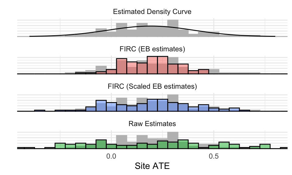
The scaled approach is closest, although the density approach also looks good in this context. The EB estimates are too peaked and close together: note the grey bars not covered by the colored bars. The raw estimates are overly scattered: note the green bars far in the tails.
The above data were generated from a normal model with all the random effects normally drawn. We next repeat the above, but for a case where the actual site-level impacts are far from normal.
Rescaling in the face of non-normality
For our second dataset, the control-side distribution is as before. The only thing we have changed is the distribution of the site-level impacts. In particular, the site impacts have a gamma distribution, with the bulk of impacts being small with a right tail of larger impacts going up to around \(0.66\sigma\) or so. For these data, the overall ATE is the same as our prior example (0.2), and the cross-site standard deviation of impacts is also the same (0.2). We calculate all estimates as we did above.
The mean and standard deviation of our site level impacts for the various methods are as follows:
| model | ATE | sd |
|---|---|---|
| Raw Estimates | 0.23 | 0.40 |
| FIRC (Scaled EB Estimates) | 0.22 | 0.26 |
| FIRC (EB Estimates) | 0.22 | 0.18 |
| true pop | 0.20 | 0.20 |
| true finite | 0.22 | 0.21 |
The scaled estimates are too scattered, indicating the FIRC model—even with 100 sites—failed to estimate the cross-site impact variation well here. We plot histograms of the three methods on top of the grey histogram of the true site-level impacts to make the character of the individual estimates more clear. The density method is completely misspecified, so we drop it from this display.
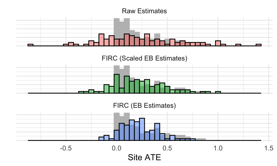
Everything has failed, and failed quite badly. The distinct shape of the original distribution of effects has been “normalized”–the measurement error coupled with the assumption of a normal distribution of effects means the final EB estimates end up with a fairly normal shape, and rescaling does not change that shape. The dispersion of the raw estimates gives a substantial share of apparent negative impacts (there should be none), but perhaps suggests the skew a tiny bit. There is some skew preserved in the FIRC and scaled FIRC estimates, which is the only good sign in a fairly bleak picture.
And only a few sites?
If we only have a few sites, but they are larger, choices between approaches become less important. The reason is that, with larger sites, we actually know the answer for the sites just by looking at the site data. In this case, just using raw site estimates is reasonable, and the shrinkage from Empirical Bayes will be less severe since site-level precision will be high (so the shrunk estimates will then basically be the same as the unshrunk).
To illustrate, we use the same skewed model, but with only 30 sites ranging in size from 250 to 1000. We have the following:
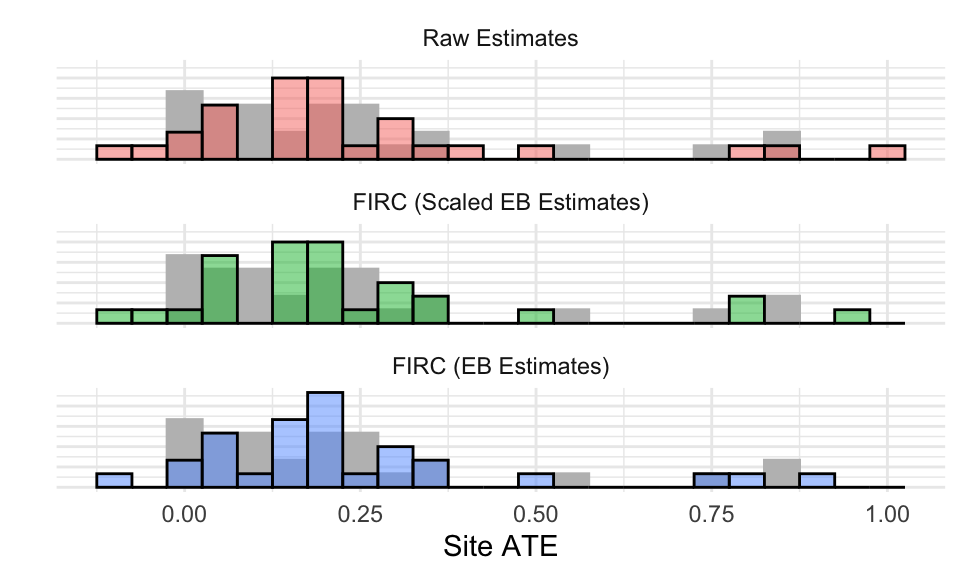
We are getting the outliers, for the most part. You can see how, for EB, they are pulled towards the center. But because the estimated center is positive, the near-zero estimates are also getting pulled up, when we know that in truth they are smaller (note how the raw approach has more mass near zero than the EB or Scaled).
We can also see how well we estimated the center and spread with our smaller sample:
| model | ATE | sd |
|---|---|---|
| Raw Estimates | 0.24 | 0.25 |
| FIRC (Scaled EB Estimates) | 0.24 | 0.24 |
| FIRC (EB Estimates) | 0.24 | 0.23 |
| true pop | 0.20 | 0.20 |
| true finite | 0.22 | 0.24 |
Our measure of spread is a bit off from the superpopulation: it is not estimation error that is causing trouble here, it is the fact that our sample that we are estimating on is not perfectly representative of the superpopulation. Different finite samples will vary in their true heterogeniety, depending on what we get. That being said, we are estimating the finite-population spread fairly well. See Bloom and Spybrook (2017) for more discussion of estimating \(\tau\), and representativeness of the finite population to super.
Conclusions
Estimating distributions is really, really hard, but we want to look at them all the time anyway. In the case of a multi-site trial, looking at the raw estimates can be deceiving—they are often over-dispersed. Looking at the shrunken estimates from Empirical Bayes is also deceiving—they are too close together. Rescaling the EB estimates can help a lot—but only if the true distribution looks about normal in the first place. Of the collection of bad options, rescaled EB is generally best. That said, in some cases more technical approaches as described in Lee et al. (2024) could help.
One might reasonably ask how much the different choices matter in practice. It can matter a lot. The amount of “fuzz” in the measurement of the individual sites drives everything. Having bigger sites, or the ability to measure impacts in a site with high precision (e.g., due to having a strongly predictive covariate), greatly improves the plausibility of the final plotted figure. Our paper, Lee et al. (2024), talks about this “fuzz” in terms of the information we have about the site-level impacts; some comprehensive simulations there show when we can and should not engage in this sort of activity.
Also in Lee et al. (2024) we try to do better job with non-normal distributions by fitting Bayesian models with more flexible forms on the distribution of the site-level impacts. These models all suffer from the overall difficulty of the problem, in that separating out the measurement error from the underlying distribution we are trying to estimate is hard: it is like focusing a blurry picture when you don’t know what the picture is of. But these more flexible approaches do prove to be beneficial in high information contexts (big sites, many sites, good predictive covariates).
Everything discussed here directly connects to meta-analysis as well. A multisite trial is simply a very clean meta-analysis where we have the raw data, but the principles of plotting and rescaling discussed above all carry over. In meta-analysis, people often make forest plots, showing the estimated impacts of each study. If they are reported raw, they are over-dispersed, just as above; just look at the trees, and do not trust your impression of the forest. Adjustments such as the above could be made, at which point the Normality assumption will rear its head, just like here. See Jackson and White (2018) for a treatment of the various ways Normality assumptions, among other things, can distort meta-analysis results.
Acknowledgements
Thanks to Jonathan Che and Mike Weiss for their thoughts and edits on this post; thanks especially to Mike for some snippits of text that I have, in effect, stolen. Deep thanks to my co-authors and collaborators on Lee et al. (2024), especially JoonHo Lee and (again) Jonathan Che, for being part of the larger and deeply interesting exploration that started many, many years ago. After an incredible number of simulations, interesting side-quests, and various meaning-making sessions, I have, due to their work, ended up with a bit more understanding of all these moving parts!