
Drawing a Line Between Sample Statistics and Population Inferences
by Eddie KimA shady figure presents you with a game. They have a deck of cards numbered 1, 2, 3, or 4, the exact distribution of which you do not know. They randomly shuffle and separate the deck into two equally sized piles, facedown, and after checking the piles for themselves, reveal some cards from each. From the first set: 4, 3, 3, 2, 2. From the second set: 4, 4, 1. The game is thus: which card pile has the higher total value?
To statisticians, this can sound like a straightforward question. The observed sample averages for the two piles are 2.8 and 3 respectively. Though the difference is slight, and the results not guaranteed, our trust in expected values and the law of large numbers should encourage us to guess the second set has the higher average card value. That is, across many similar encounters, with similarly shady figures, we would expect to win the game more often than not using such a strategy.
But this reasoning is vulnerable to exploitation, particularly from, say, figures thusly shady. Though tempting, we could not assume that the revealed cards were chosen at random; that was never established. If we knew for a fact that the shady figure deliberately chose to reveal the highest value cards in each pile, we could definitively conclude that the first pile has the higher total value. The lesson of this story is not whether the player should guess the first or second set, but rather that the question is not straightforward. Failing to recognize what one took for granted turns the player into a mark, and the game into a con.
Real life examples of this dynamic are quite common. Alabama’s average reported SAT score in 2019 among high school graduates was 1143 versus 1120 for Massachusetts, but no education researcher would seriously consider this proof that in general Alabama students outperform Massachusetts students at math and reading (note that only 7% of Alabama’s graduates took the SAT compared to 81% of Massachusetts’s graduates). Whenever observations from distinct groups selectively (i.e., non-randomly) enter into the sample according to different patterns, any sample statistics will capture and describe inherently different parts of the underlying populations, distorting population comparisons. Employing clever statistical methods in these situations can still permit accurate conclusions. One well-known tactic is to compare in-sample versus out-of-sample demographics to determine, and then correct for, any selection into sample mechanisms based on demographics (Heckman, 1979; Cuddeback et al, 2004). But this information is not always available, especially when one is reading the research rather than conducting it for oneself.
A method I have developed (read: “am currently still preparing for publication”) for such circumstances is a procedure I call Reverse Sample Selection Speculation (RSSS). Importantly, RSSS relies on just three observed facts: population size, sample size, and a sample level summary statistic. The core idea is that even if we may not know exactly how a population selects into an observed sample, we can often make an educated guess as to a plausible scenario (e.g., higher performing students are more likely to sit for the SAT exam). We can then pair this with a null hypothesis (e.g., Alabama students have equal SAT scores to Massachusetts students in the population) and then determine the likelihood that we would observe the given sample statistics under the chosen scenario and hypothesis. By considering the combinations of multiple scenarios and null hypotheses, we can qualify each potential population inference, as in the example table below.
RSSS can reveal alternative lines of investigation to address the original research question (e.g., exactly how much more likely are higher performing students to sit for the SAT exam?), or disqualify some null hypotheses altogether (e.g., because we know that higher performing students are at least somewhat more likely to sit for the exam, we can conclude Alabama and Massachusetts SAT scores are not equal in the population).
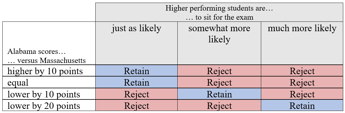
An example matrix of scenarios and null hypotheses; results are hypothetical and not the result of actual calculations
Let’s try a casual, low-stakes example.
Start with the Facts
In 2014, Students for Fair Admissions (SFFA) sued Harvard College alleging that Harvard illegally discriminated against Asian American applicants. One of the arguments that SFFA brought forward in the case was the distribution of Personal ratings by race. The Personal rating considers “such traits as whether the student has a ‘positive personality’ and ‘others like to be around him or her,’ … is ‘widely respected,’ is a ‘good person,’ and has good ‘human qualities’” (see SFFA’s Motion for Summary Judgement). Though Personal ratings range from 1 to 5 in practice, in its presented evidence SFFA bins them into what I will refer to as “high”, “medium”, and “low” categories, with the distributions, as categorized by the report, as follows:
| Group | N | “High” Personal Rating | “Medium” Personal Rating |
|---|---|---|---|
| Asian American | 40,308 | 17.64% | 81.88% |
| White | 57,451 | 21.27% | 78.30% |
| African American | 15,601 | 19.01% | 80.52% |
| Hispanic | 17,930 | 18.68% | 80.85% |
Indeed, proportionally less Asian applicants received a high Personal rating as compared to applicants of other racial groups. We can also phrase this in terms of quantiles. Imagine that one’s Personal rating is in fact a perfectly continuous variable (i.e., not binned strictly into 1 through 5), and for simplicity consider the Asian American group versus the African American group. Though we do not have precise numbers for each applicant’s Personal rating, we do observe that there exists some cutoff for a “high” Personal rating, and 17.64% of Asian American applicants passed that cutoff whereas 19.01% of African American applicants did the same. Thus, in the observed sample, the 82.36th quantile of Asian American applicants equals the 80.99th quantile of African American applicants; for a given caliber of African American applicant, one need look higher on Asian Americans’ sample distribution to find a comparable applicant. But is this proof of racial discrimination?
Asking that question (and expecting a useful answer) at this point betrays a litany of logical legerdemain. First, proving racial discrimination in this context is ultimately a legal question; SFFA’s case against Harvard touched on many topics and using statistics to compare applicant Personal ratings was only one piece of a much larger trial. What a statistical inquiry can contribute is evidence of discrimination: does Harvard College’s evaluation of Asian Americans seem to align with how it would behave in the absence of discrimination? That is, if we can establish what nondiscrimination would look like in terms of statistics (a tenuous position which I’ll return to later), then we can assess whether the statistics we observe match up with that impression.
Second, the numbers that we are dealing with here are sample statistics, whereas any benchmark of discrimination, or lack thereof, need refer to population statistics. After all, Harvard does not control the sample it observes. Let’s say I recruited a thousand additional Asian Americans (at random) to try out for the U.S. Olympic badminton team. Even if the team’s recruitment criterion stayed the same, the admit rate of Asian Americans to the team among try-out-ee’s would likely plummet compared to previous years’ cohorts. But, the team did not become more discriminatory towards Asians; the selection into sample pattern changed. A population level comparison asks, “what would we observe if every Asian American student and every African American student applied to Harvard?”, an answer which does not change regardless of who ultimately chooses to apply. Technically, we could immediately jump from sample statistics to population inferences if we were confident that the observed samples captured similar portions of their respective populations, but that brings up the third point.
Third, the observed samples almost certainly do not capture similar portions of their respective populations. Consider the application rates to Harvard by race, a piece of information left out of SFFA’s analysis of Personal ratings. SFFA utilizes a specific mix of cohorts across years and figuring out the appropriate, aggregate application rate for this sample would be nigh impossible. However, we can infer some stand-in estimates based on publicly available information. According to SFFA’s data, the admit rate for the class of 2017 was 5.6%, 7%, 6.8%, and 6.1% for Asian, white, African American, and Hispanic applicants, respectively. The number of students in that class year who identified with these four categories according to Harvard’s administrative documents (excluding nonresident aliens and non-Hispanic two or more races) was 306, 715, 116, and 1671. Uniformly applying the average yield rate (i.e., the percent of students who enroll at Harvard after acceptance) of 82% for that year, we estimate 6,664 Asian American applicants, 12,456 white applicants, 2,080 African American applicants, and 3,339 Hispanic applicants for the class of 2017. Finally, using 12th grade enrollment numbers from the 2013 American Community Survey2, we approximate that 3.45% of all Asian American 12th graders applied to Harvard, while that figure for white, African American, and Hispanic 12th graders was only 0.42%, 0.21%, and 0.32%. That is, based on this class’s data, we approximate that Asian Americans are more than eight times as likely to apply to Harvard as students of any of the other racial groups. Clearly, the Asian Americans who apply to Harvard represent their greater population in a very different way than the African Americans who apply to Harvard represent theirs. Although it is possible for samples to differently represent their populations in a way that does not distort sample statistic comparisons such situations are exceedingly rare, and readers should treat with great skepticism arguments that take this situation as a given.
Hence, the sample statistics presented by SFFA cannot be considered even evidence of racial discrimination prima facie. While sample statistics can still inform population inferences in the face of sample selection if said sample selection mechanisms are properly accounted for, we can’t do that here. Concrete data to inform said mechanisms are absent from Harvard’s and SFFA’s documents (at least within the publicly available portions). At this point, in recognition of the mathematical deception at play, one could simply refuse to engage with the interlocutors and op-eds that harken to these Personal ratings; as tantalizingly intuitive as it may seem, the numbers simply cannot support an argument of discrimination against Asian Americans. But we can also go a step further. We can attempt to reverse the effects of sample selection, if we can tolerate some speculation, using Reverse Sample Selection Speculation. When SFFA alleges that these numbers suggest racial discrimination against Asian Americans, what are they implicitly asking the audience (or judge) to believe about how those numbers came about?
(A mild spoiler but useful scaffolding point: by the end of this inquiry, we’ll find that the logical endpoint to SFFA’s allegation requires some assumptive worldviews that are difficult to swallow, while under more reasonable positions we would actually prefer to allege in the opposite direction. The intent is neither to affirm nor deny these positions, but rather set straight which direction the data would point if we decide to follow it at all.)
What’s the Probability of Equal Means?
RSSS technically begins with speculation on the structure of the data (e.g., what shape is the unobserved population distribution). A full discussion of this topic is well beyond the scope of a blog post, but we can content ourselves here with standard normal distributions for the populations (i.e., mean 0, variance 1), and linear logistic regressions for the selection functions, canonical choices as they are for scale invariant population distributions and selection functions. Now, consider the following null hypothesis and hypothetical selection into sample pattern:
Hypothesis: The population distributions of Asian American and African
American
12th graders’ Personal ratings have equal means
distribution are 90% likely to apply to Harvard
Recall in the original card game that if we presumed a scenario where the shady figure had chosen the highest value cards to reveal, with a reveal of 4, 4, 1, we could infer the remainder of the second card pile, and we could bound our expectations of the first pile with its reveal of 4, 3, 3, 2, 2 (i.e., everything else must be 2 or 1). In a similar way, we can try on the scenario above to bound our beliefs about the Asian American and African American population distributions. After following the scenario to its logical conclusions, we can then consider alternatives and delineate what kind of realities would support which inferences.
In canonical statistics fashion, we will first consider that the sample statistics we observed came from a world where the null hypothesis is true (populations have equal means), then calculate the actual probability that such statistics would have occurred from such an assumed world. If we find that that probability is very low, we can conclude that the assumed world, with its equal means, is in fact not the world that generated these observations; we would otherwise need to conclude that we have experienced a very low probability event. In our case, we are considering the circumstance that the 82.36th percentile of the Asian American sample equals the 80.99th percentile of the African American sample. How likely was that to occur?
We already have enough information to uncover some concrete numbers. Our sample selection function (a linear logistic regression) must calibrate its slope and intercept parameters such that, for a standard normal population distribution, we would expect 3.45% of the population to enter the sample and for individuals at the 99.9th percentile to be 90% likely to apply to Harvard. Numeric integration and an optimization procedure make quick work of this two-unknowns-two-equations context (slope = 2.56, intercept = -5.70). And, we can do the same for the African American population Personal ratings (slope = 11.47, intercept = -33.26).
Now we can map out the theoretical sample distributions for Personal ratings. We know that 17.64% of the observed Asian American sample passed the benchmark of a “high” Personal rating. So, what is that benchmark value? What number would we expect exactly 17.64% of this sample to surpass? Using our selection functions, population distributions, and a well-known mathematical property of sample quantiles3, we can calculate that the 82.36th percentile for the Asian American sample, which we’ll denote λA, is expected to be 2.41, with a standard error of 0.0049. Across many theoretical samples, the exact value of λA may differ due to random fluctuations in applicant behavior, but we wouldn’t expect it to vary by much given such a large sample and such a small standard error. So, our best estimate, based on the sample statistics of Asian Americans, is that students need an internal Personal rating of at least 2.41 (on our hypothetical continuous scale) to receive a “high” Personal rating (on SFFA’s interpretation of the admission office’s scale). And because we started with standard normal populations, we can interpret this to mean only students 2.41 standard deviations above the mean, the top 0.8% percent, would score a “high” Personal rating if they applied to Harvard, consistent with the fact that of Asian Americans 3.45% applied, and of that sample only 17.64% scored a “high” Personal rating.
We can perform a parallel analysis to determine that the expected value corresponding the 80.99th percentile for the African American sample, λB, is 3.35 (with an associated standard error of 0.0046). So, our best estimate, based on the sample statistics of African Americans, is that students need an internal Personal rating of at least 3.35 to receive a “high” Personal rating. Because we started with standard normal populations, we can interpret this to mean only students 3.35 standard deviations above the mean, the top 0.04%, would score a “high” Personal rating if they applied to Harvard, consistent with the fact that of African Americans 0.21% applied, and of that sample only 19.01% scored a “high” Personal rating.
Something is clearly amiss. All our calculations thus far were the logical ramifications of our starting conditions and sample data which noted that the same benchmark value demarcated 17.64% and 19.01% of the two samples. However, the analysis suggests that not only do we expect the two benchmark values to be different in practice, but further that we would be extremely surprised if they were in fact the same. Back to canonical statistical inference: we therefore reject the null hypothesis that the Asian American and African American population distributions have equal means, and further, we reject this hypothesis in favor of Asian Americans having a higher population mean. In other words, based on the observed data, our assumptions of data structure, and this scenario constraint, if every 12th grader in the U.S. applied to Harvard College, we would expect overall that Asian Americans applicants would score higher on the Personal rating than African American applicants. If our standard for racial non-discrimination on the part of Harvard College was that the population means were equal, we would indeed suspect discrimination had taken place, but discrimination in favor of Asian American applicants.
We can use the same procedure with other scenarios as well (let’s call the first scenario introduced Scenario A). Consider:
Asian Americans below the 96.55th percentile, and African Americans lower than the 99.79th percentile, on their respective population distributions have at most a 25% chance of applying to Harvard
The top 3.45% of Asian Americans on the Personal rating distribution compose 80% of Asian American applicants; the top 0.21% for African Americans
The bottom 90% of each population distribution composes 5% of the applicant pool
Note that all four of these scenarios are hypothetical, speculative – four interpretations of the intuition that students with higher Personal ratings are more likely to apply to Harvard College4 and the mathematical limits of a 3.45% and 0.21% application rate. I encourage curious readers to consider other constraints and scenarios of their own. However, a telling result is that across all four of these we arrive soundly at the same conclusion: the population means are not the same, in favor of Asian Americans having a higher population mean.
| Scenario A | Scenario B | Scenario C | Scenario D | |
|---|---|---|---|---|
| Expected value of \(\lambda_A\) | 2.41 | 2.39 | 2.5 | 2.49 |
| Standard Error of \(\lambda_A\) | 0.0049 | 0.005 | 0.0038 | 0.004 |
| Expected value of \(\lambda_B\) | 3.35 | 3.31 | 3.35 | 3.2 |
| Standard Error of \(\lambda_B\) | 0.0046 | 0.0056 | 0.0046 | 0.0071 |
| Expected difference in SD units | -140.78 | -121.97 | -142.26 | -87.04 |
| p-val of \(\lambda_A = \lambda_B\) | \(\approx 0\) | \(\approx 0\) | \(\approx 0\) | \(\approx 0\) |
So Which Hypotheses are Probabilistically Believable?
To be fair, this is not specifically SFFA’s claim of racial discrimination. Though they clearly object to the fact that 17.64% of Asian American applicants and 19.01% of African American applicant received “high” Personal ratings (i.e., the 82.36th percentile for the Asian American observed sample is equal to the 80.99th percentile for African Americans observed sample), it is not apparent what counterfactual they are arguing for. One possible position is that even though the observed statistics would suggest Asian Americans generally have higher Personal ratings than applicants of other racial groups, in reality the population level differences are even greater. (The Boston Celtics should obviously win against my middle school team, but we would still raise eyebrows if they only won by a few points.) SFFA implies this when they point out that among students with comparably high academic achievement the Asian American applicants are assigned lower Personal ratings. Underlying this statement is the assertion that because Asian American applicants have higher academic scores, they should also have similarly higher Personal ratings, otherwise they are victims of discrimination. However, this inference is flawed. Even if correlations between academic prowess and Personal rating were identical across racial groups, sample selection on academic ability could produce the same observed pattern of a lower proportion of high Personal ratings within the observed sample, and an even lower proportion among the high Academic rating scorers in the observed sample.
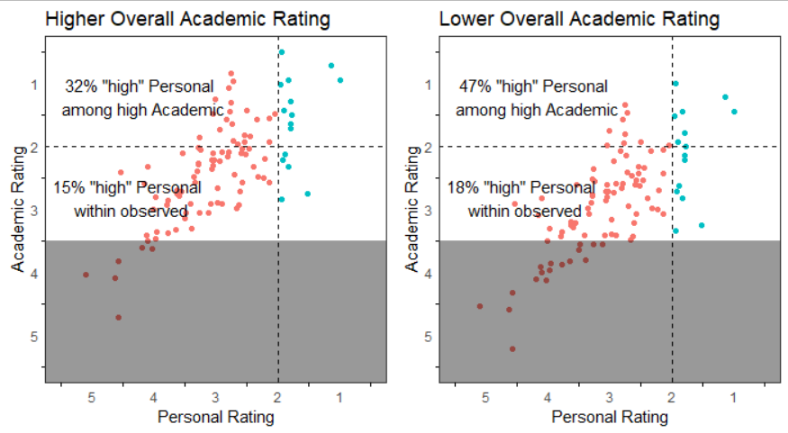
Figure 1: The white area represents students who entered the observed sample versus the darker area of students who did not. The RHS observed sample has a higher proportion of high Personal ratings versus the LHS observed sample, but this is an artifact of fewer low Personal rating students entering the RHS sample, due to their concurrent low Academic rating, rather than a difference in Personal rating distributions. This pattern is exacerbated within the high Academic rating subset, which filters further for high Academic rating regardless of Personal rating. Note that the LHS and RHS observations are identical but for a vertical (i.e., Academic rating) shift; each has the same number of high Personal rating students in the population.
Thus, the position that Asian American applicants do have higher Personal ratings in the population is a hypothesis, and one that we can test. To recap, our objective now is to investigate the claim that Asian Americans are underperforming relative, not to other racial groups, but to expectation. That is, what if in truth λA exceeds λB by some margin x, but the sample statistics only suggest a margin of x’, where x’ < x? Fear not. In the same way that we previously used RSSS to test the one null hypothesis of equal population means, we can use RSSS to calculate the suggested difference in population means x’ by finding which range of null hypotheses we cannot reject at the 0.05 level. We will fix the African American population to the same standard normal, but the Asian American population distribution will be a normal distribution of variance 1 and various means. The table below displays the results with three rows: the lowest value for x’, the presumed difference in population means, for which we could not reject the null hypothesis; the expected value for x’ given the sample statistics; and the highest value for x’.
| x’ Value | Scenario A | Scenario B | Scenario C | Scenario.D |
|---|---|---|---|---|
| Lowest non-reject value of x’ | 1.85 | 1.75 | 2.07 | 1.76 |
| Most likely value for x’ | 1.87 | 1.78 | 2.09 | 1.79 |
| Highest non-reject value of x’ | 1.90 | 1.80 | 2.12 | 1.82 |
We can now formally quantify the position that given the observed Personal rating data one should conclude discrimination against Asian American applicants, the position which SFFA appears to argue from. For example, if we abide Scenario A, we must first believe that on average Asian American 12th graders’ Personal ratings are nearly two standard deviations higher than African American 12th graders’ to then construe the observed sample statistics as evidence of racial discrimination against Asian Americans; less than that and we would rather conclude in the opposite direction.5 Or, said another way, if anyone chooses to conclude that Harvard did discriminate against Asian Americans based on the observed statistics, then they must implicitly believe that less than 3% of African American 12th graders are on par with the average Asian American 12th grader.
To be clear, population level differences in Personal rating between racial groups likely do exist, the same way there demonstrably exist Academic, Extracurricular, and Athletic rating differences.6 Racism, resource disparities, societal pressures and expectations, snake oil salespersons, and cultural differences all conspire to nudge high school students in various directions based on their race and ethnicity, and prompt colleges to reward certain accolades and mannerisms while looking poorly upon others.7 I am not arguing that the statistics compiled by SFFA represent ratings that are free of any racial bias. Rather, I am arguing that to bandy about that data as evidence of discrimination without acknowledging the priors that that position presupposes is irresponsible.
Watch the Dealer, Not the Cards
As stated at the outset, this statistical investigation cannot prove discrimination one way or another. That is not the objective of RSSS. The approach of Reverse Sample Selection Speculation is, inherently, speculative. On the one hand, one must infer or intuit the functional forms, scenarios, and parameters. The values I chose and decisions I made are likely easily refuted by anyone with access to SFFA’s detailed files. But on the other hand, the fact that, under reasonable choices and assumed group equality, statistical probability suggests we would rather conclude Asian American applicants were discriminated for than against places the burden of evidence on the claimant who alleges otherwise. If one is to interpret this data at all, one must do so correctly.
Despite my intention to present RSSS as colloquially as possible, not everyone will have the foundational knowledge to fully grasp all its mechanics. The actual statistical underpinnings of RSSS are quite complex and I hope I have left enough details (and would be happy to provide more) for other statisticians to validate, reproduce, and extend the ideas I’ve presented herein. But the core logic of RSSS and the trickery it exposes are quite accessible, and I encourage every responsible consumer (and creator) of statistical evidence to remain vigilant. Are we being asked to compare samples or populations? How similarly do the observed statistics represent their respective populations?
We must be wary of those who would hastily draw lines between sample statistics and population inferences, and shady figures who would encourage us to study the revealed cards but overlook how the cards were chosen from the deck.
Image credit: Thumbnail image from Pixabay
See: https://oir.harvard.edu/files/huoir/files/harvard_cds_2013-14.pdf↩︎
Steven Manson, Jonathan Schroeder, David Van Riper, Tracy Kugler, and Steven Ruggles. IPUMS National Historical Geographic Information System: Version 17.0 \[dataset\]. Minneapolis, MN: IPUMS. 2022. http://doi.org/10.18128/D050.V17.0↩︎
The sample distribution for \(\widehat{\lambda_{A}}(q)\) is:
\(N\left( \lambda_{A}(q),\ \frac{q(1 - q)}{n\ \left\lbrack \delta_{A}\left( \lambda_{A}(q) \right) \right\rbrack^{2}} \right)\),
where δA is the p.d.f. of the sample distribution for group A, n is the sample size for group A, and λA(q) is the inverse of the cumulative density function corresponding to δA.↩︎
We can also point to empirical data. Evidence brought forward by SFFA shows that the Personal rating is positively correlated with academic ability, and empirical patterns from data sets such as the High School Longitudinal Survey make clear that higher academic ability students are more likely to apply to highly selective institutions such as Harvard College.↩︎
The exact maths for the relationship between the boundary x’ values and scenario details are beyond the scope of this post. However, in general, the more selective group A’s observed sample is to its population, especially versus how group B’s observed sample is to its population, the greater the expected value for x’. For example, for Scenario A, if the 99.9th percentile were more than 90% likely to apply, the expected x’ values would be greater.↩︎
Comparing Asian Americans to any other racial group results in similar conclusions. If we run the same analysis comparing African American to Hispanic students, we also see significant deviations from the null of equal population means, but the suggested boundary values x’ generally correspond to less than a standard deviation in magnitude.↩︎
I was diligently assured by my Korean immigrant parents that my golden ticket to a prestigious college was through studying very, very hard for the SAT, diligently assured as they were by friends, family, and peddlers of SAT prep books and tutoring services. However, that is a story for another time.↩︎