Exploring power with the PUMP package
by Luke MiratrixThere are a lot of ways to do power calculations, but I wanted to show off a package, PUMP, that my collaborators and I recently set out into the world.
The original purpose of the package was to provide tools for power analyses that account for multiple outcomes under a variety of common experimental designs—an awesome purpose that I was pleased to be a part of—but as a result of our trying to make everything as user-friendly as possible, we ended up with a package that has some nifty bells and whistles even for single outcome power analyses.
And single outcome power analyses is what this blog post is about.
If you want more on the multiple outcome use of PUMP, check out the MDRC introductory blog and demo (link), our just accepted Journal of Statistical Software paper (Hunter, Miratrix, and Porter (2021) (link)), and the website that wraps the package in a Shiny app to make a web interface (link).
With regards to a single outcome, there are two things I really love about PUMP.
The first is our technical appendix, where we tried to generate an ontology of different designs (cluster-randomized experiments, multi-site randomized trials, etc.) and models (fixed effects models, the FIRC, or fixed-intercept, random coefficient model, etc.), with formulae for the standard errors for each.
In education (and many other places besides) randomized field trials often have very specific structure to account for the realities of implementing new programs.
For example, we might randomize schools, but look at student outcomes (i.e., a cluster randomized experiment, with the schools being the clusters).
Or we might randomize first gen students within a set of community colleges to receive extra supports or not (i.e., a multi-site randomized experiment, with the colleges being the sites).
In particular, we separate the experimental design (e.g., it’s a multisite randomized trial) from the planned model for analysis (e.g., we will estimate impacts with a linear regression with fixed effects). This separation draws attention to the consequences of treatment impact variation and whether one is targeting a superpopulation or finite population quantity, which is a pet interest of mine. See, for example, Miratrix, Weiss, and Henderson (2021), which explores the consequences of choosing across more than a dozen methods of analyzing multisite experiments. Also see co-author Kristen Hunter’s “10 things you should know” piece on multisite experiments more generally (link).
Anyway, like many power calculaters (e.g., PowerUp!), PUMP (the Power Under Multiplicity Project) supports these designs, and our technical appendix tries to organize them in a systematic way, defines a naming scheme for designs and models, and provide some technical details.
You can find the appendix starting on page 30 of our ArXiV pre-print.
I find myself using the technical appendix as a reference for different experimental contexts all the time; for example, if I want to remind myself of how to calculate needed site size or number of sites for a multisite experiment, I can easily look it up.
The second thing I love about PUMP is the ability to explore a lot of different design parameters all at once, and to make plots nearly automatically.
This automation allows for rapid exploration and sensitivity checks on an initial analysis.
I will mainly focus on this fanciness below.
The PUMP pacakge is posted on CRAN, or you can install the most recent version from GitHub via:
devtools::install_github( "https://github.com/MDRCNY/PUMP" )The three core methods for PUMP are pump_power(), pump_sample(), and pump_mdes(), for calculating power given a specific effect size, how many units we would need to be well powered for a specified effect size, and the minimum effect size we could reliably detect given a desired power, respectively.
For a running example, say we have a multisite randomized trial with 20 sites with an average of 80 students per site. We plan on treating 50% of the students in each site and we want to know the smallest impact (in effect size units) we could reliably detect. We can rely on defaults and write:
library( PUMP )
res <- pump_mdes( "d2.1", nbar = 80, J = 20,
                  Tbar = 0.50,
                  target.power = 0.80 )
## Warning: Selecting design and model d2.1_m2fc as default model for design from
## following options: d2.1_m2fc, d2.1_m2ff, d2.1_m2fr, d2.1_m2rrLet’s dissect the above call.
The d2.1 specifies the design, which in this case is two-levels, with randomization at level 1 (i.e., a multisite randomized trial).
Because we didn’t specify one, the package then picked a default model, i.e., it picked how we would analyze our data, once we had it.
The model syntax is a pair of letters denoting whether we have fixed, random, or constant intercepts and treatment impacts at level 2.
The default here is a fixed intercept and a single constant treatment impact coefficient, or m2fc.
The nbar is the average number of students per site, and J the number of sites. Tbar is proportion treated.
We can look at the results as follows:
summary( res )## mdes result: d2.1_m2fc d_m
##
## target D1indiv power: 0.80
## nbar: 80 J: 20 Tbar: 0.5
## alpha: 0.05
## Level:
## 1: R2: 0 (0 covariates)
## 2: fixed effects ICC: 0 omega: 0
## rho = 0
## MTP Adjusted.MDES D1indiv.power
## None 0.1401658 0.8
## (max.steps = 20 tnum = 1000 start.tnum = 100 final.tnum = 4000 tol = 0.02)We see that if the true treatment impact were around 0.14 or larger, we would have at least 80% power to detect it, given our experimental design and modeling choices.
If we also estimate that our (level 2) intra-class correlation (ICC) is 0.20 and that we can improve precision with 5 predictive baseline covariates with an overall \(R^2\) of 0.60, we can include that additional information easily:
res2 <- pump_mdes( "d2.1_m2fc", nbar = 80, J = 23,
                   Tbar = 0.50,
                   R2.1 = 0.60, numCovar.1 = 5,
                   ICC.2 = 0.20,
                   omega.2 = 0.4,
                   target.power = 0.80 )
print( res2 )
## mdes result: d2.1_m2fc d_m
## target D1indiv power: 0.80
## MTP Adjusted.MDES D1indiv.power
## None 0.07393223 0.8Our ICC and covariates have reduced our MDES substantially.
In the above call we have thrown in some treatment effect variation via omega.2 as well—omega.2 is the ratio of the variance of the site-level treatment impact to the variance in the random intercepts.
Playing with specifications
We can easily play with different configurations via the update() method.
Here, for example, we reduce the number of people per site, and increase the number of sites:
update( res2, nbar = 20, J = 80 )## mdes result: d2.1_m2fc d_m
## target D1indiv power: 0.80
## MTP Adjusted.MDES D1indiv.power
## None 0.07929187 0.8Our MDES is basically unchanged!
This kind of haphazard exploration can be useful for quick questions, but sometimes it is worth exploring more systematically.
Systematic exploration is where PUMP really shines.
For example, we can rapidly explore a bunch of different combinations of number of sites and sizes of sites via the update_grid() function, which will look at all combinations of lists of passed parameters:
grd = update_grid( res2,
                  J = c( 20, 80 ),
                  nbar = c( 20, 80 ) )
grd
## mdes grid result: d2.1_m2fc d_m
## Varying across J, nbar
## MTP d_m J nbar Adjusted.MDES D1indiv.power
## None d2.1_m2fc 20 20 0.15889598 0.8
## None d2.1_m2fc 20 80 0.07928992 0.8
## None d2.1_m2fc 80 20 0.07929187 0.8
## None d2.1_m2fc 80 80 0.03962652 0.8You can also update entire grids. For example, let’s look at using the so-called FIRC (Fixed Intercept, Random Coefficient) multilevel model as an analytic plan, and compare MDESes between the two.
grd2 = update_grid( grd, d_m = "d2.1_m2fr" )
grd2
## mdes grid result: d2.1_m2fr d_m
## Varying across J, nbar
## MTP d_m J nbar Adjusted.MDES D1indiv.power
## None d2.1_m2fr 20 20 0.25564808 0.8
## None d2.1_m2fr 20 80 0.20873578 0.8
## None d2.1_m2fr 80 20 0.12045065 0.8
## None d2.1_m2fr 80 80 0.09834754 0.8We are seeing substantial increase in the MDES; this is the super-population vs. finite population tension mentioned above.
The increase is because FIRC allows for cross-site impact variation, and views the sites in our experiment as a sample of a larger superpopulation.
The increase captures the additional uncertainty of the experimental sample being representative of this larger population.
Our original m2fc model does not allow for this variation, and thus is implicitly estimating the finite-sample average treatment effect, which is an easier goal.
See Miratrix, Weiss, and Henderson (2021) for further discussion.
PUMP makes exploring such choices and trade-offs readily apparent.
This tension is one reason why we tried to separate the design and model so explicitly as well.
If we turn to plotting, we can explore many scenarios at once:
grd3 = update_grid(grd2,
                   J = c( 20, 25, 30, 35, 40),
                   nbar = seq( 20, 75, by = 5 ) )
plot( grd3, var.vary = "nbar", color = "J" ) +
    geom_hline( yintercept = 0.20 )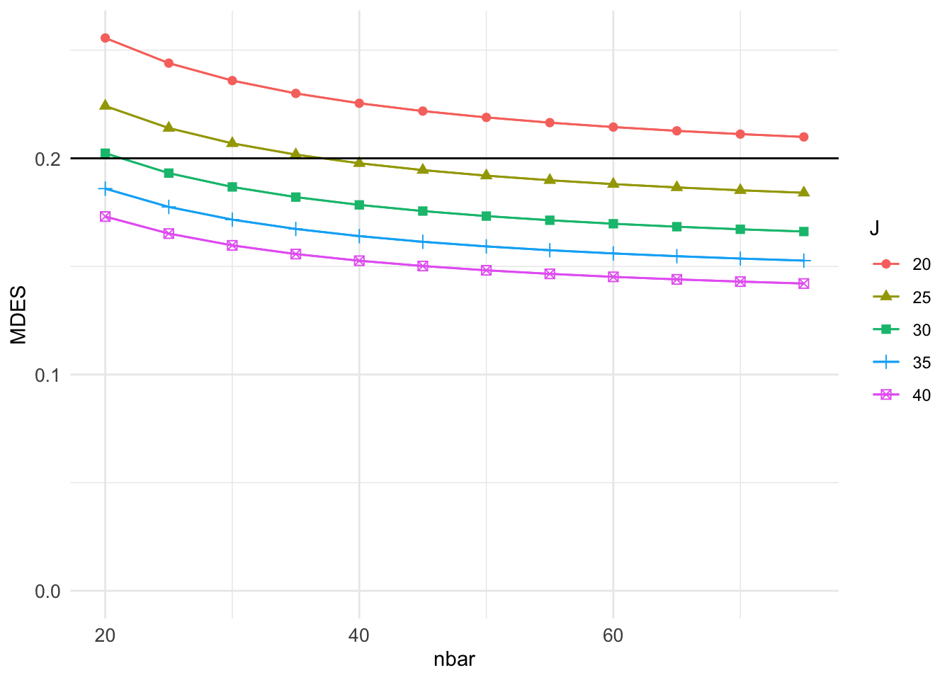
In the plot command, we specify the \(x\)-axis with var.vary = "nbar" and the grouping by color with color = "J".
Given these settings, we have lines corresponding to the different numbers of sites examined, and we can see how MDES (\(y\)-axis) depends on nbar (\(x\)-axis) given those numbers.
Digging into the results
A pump result object is also a data.frame object, so you can work with it in that form.
For example, here I filter out those experiments with 1000 total units to see how size of site vs. number of sites plays out:
grd3 %>%
    mutate( N = nbar * J )  %>%
    filter( N == 1000 ) %>%
    dplyr::select( -MTP, -d_m, -N, -D1indiv.power ) %>%
knitr::kable( digits = c(0,0,2) )| J | nbar | Adjusted.MDES |
|---|---|---|
| 20 | 50 | 0.22 |
| 25 | 40 | 0.20 |
| 40 | 25 | 0.17 |
It apparently is better to have more clusters of smaller size, than fewer clusters of larger size.
Because these pump results are data frames, making custom plots is much easier. To illustrate, let’s explore the cost of superpopulation inference (see Miratrix, Weiss, and Henderson (2021), again, for further discussion). We are first going to make a grid where we vary the modeling choice, the sample sizes, and impact variation. We then make a customized plot of the percent increase in MDES (near equivalently, standard error) for our superpopulation estimator as compared to our finite population.1
First, our grid:
big_grd = update_grid( grd3,
                       d_m = c("d2.1_m2fr", "d2.1_m2fc" ),
                       nbar = seq( 20, 100, by = 20 ),
                       J = seq( 10, 40, by = 10 ),
                       ICC.2 = 0.2,
                       omega.2 = c( 0, 0.1, 0.2, 0.5 ) )
Next, our plot:
ggplot( big_grd, aes( omega.2, Adjusted.MDES, group = J, col=as.factor(J) ) ) +
    facet_grid( d_m ~ nbar, labeller = label_both ) +
    geom_line() +
    geom_hline( yintercept = 0.2 ) +
    labs( title = "MDES for finite population and superpopulation estimators",
          color = "J", y = "Adjusted MDES", x = "individuals/cluster" )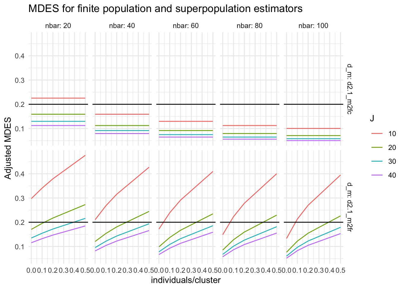
We see that for finite-sample inference (top row) the amount of treatment variation (\(x\)-axis) does not matter, but if we are generalizing to a super-population, more treatment variation means more difficulty powering to detect an average effect due to the additional uncertainty in whether the sample is representative of the population.
We can easily manipulate our results to focus on percent increase in the standard error of a superpopulation estimation vs. finite population:
big_grd_w <- big_grd %>%
    pivot_wider( names_from = d_m, values_from = Adjusted.MDES ) %>%
    mutate( inflation = d2.1_m2fr / d2.1_m2fc - 1)
ggplot( big_grd_w, aes( nbar, inflation, group = J, col=as.factor(J) ) ) +
    facet_wrap( ~ omega.2, nrow=1, labeller = label_both ) +
    geom_line() +
    geom_hline( yintercept = 0 ) +
    scale_y_continuous(labels = scales::label_percent(scale = 100)) +
    labs( title = "Percent increase in standard error of superpopulation vs. finite",
          color = "J", y = "Percent increase in SE", x = "individuals/cluster" )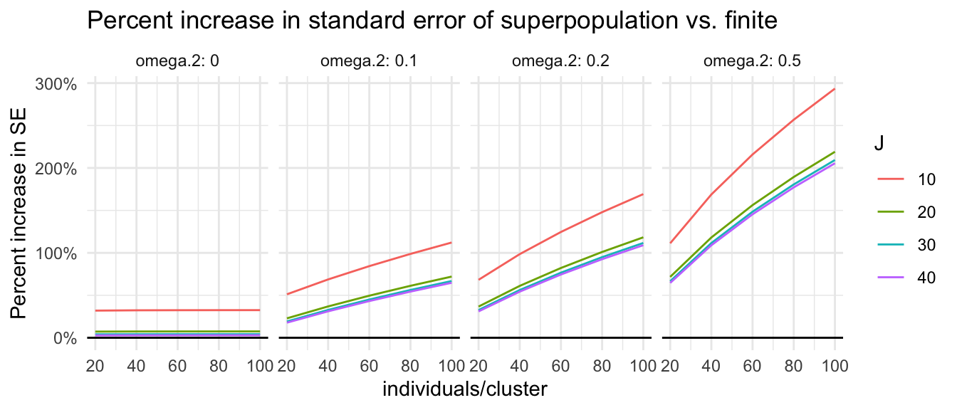
For many plausible experiments (e.g., 20 clusters with 80 units per cluster, when \(\omega_2=0.2\)), the superpopulation standard errors can easily be twice as big (100% inflation). The cost of generalization is high.
What about actual power?
I usually think in terms of MDES, but sometimes we just want to know how powerful a given experiment is.
Calculating power is easy to do via pump_power().
For example, say we are curious about an experiment with \(K=10\) blocks, \(J = 6\) clusters per block, and \(\bar{n}=50\) individuals per cluster:
initial_experiment = pump_power( d_m = "d3.2_m3ff2rc",
                                 MDES = 0.20,
                                 nbar = 50, J = 6, K = 10,
                                 Tbar = 0.50,
                                 ICC.2 = 0.2, ICC.3 = 0.2,
                                 R2.1 = 0.6, R2.2 = 0.5,
                                 omega.2 = 0.2, omega.3 = 0.2,
                                 numCovar.1 = 5, numCovar.2 = 5 )
summary( initial_experiment )
## power result: d3.2_m3ff2rc d_m
##
## MDES vector: 0.2
## nbar: 50 J: 6 K: 10 Tbar: 0.5
## alpha: 0.05
## Level:
## 1: R2: 0.6 (5 covariates)
## 2: R2: 0.5 (5 covariates) ICC: 0.2 omega: 0.2
## 3: fixed effects ICC: 0.2 omega: 0.2
## rho = 0
## MTP D1indiv SE1 df1
## None 0.641 0.084 35
## (tnum = 10000)We have about 64% power. We also see our standard error is 0.08. How much larger of an experiment would we need to get that to 80?
And needed sample sizes?
A final note is we can calculate needed sample sizes, holding other sample sizes constant. For example, for a blocked, cluster-randomized experiment we can ask how many blocks, clusters, or individuals per cluster we need.
Continuing the above, we can see how many blocks (\(K\), level 3) are needed to get to 80% power (given \(J=6\) and \(\bar{n} = 50\)):
update( initial_experiment, type="sample",
        typesample = "K", target.power = 0.80 )
## sample result: d3.2_m3ff2rc d_m
## target D1indiv power: 0.80
## MTP Sample.type Sample.size D1indiv.power
## None K 14 0.8Or see how many additional clusters per block (level 2) are needed:
update( initial_experiment, type="sample",
        typesample = "J", target.power = 0.80 )
## sample result: d3.2_m3ff2rc d_m
## target D1indiv power: 0.80
## MTP Sample.type Sample.size D1indiv.power
## None J 9 0.8Or see if we could just increase the cluster sizes:
update( initial_experiment, type="sample",
        typesample = "nbar", target.power = 0.80 )
## Warning: Cannot achieve target power with given parameters.## sample result: d3.2_m3ff2rc d_m
## target D1indiv power: 0.80
## MTP Sample.type Sample.size D1indiv.power
## None nbar NA 0.8In the final case, the warning is telling us that, even with infinite size clusters, we would not be able to achieve the desired power. This inability is because of the level 2 variation: treatment being assigned at level 2 means the number of level 2 units is driving a lot of our uncertainty, regardless of their size.
Final thoughts
Power analyses are, by their nature, exercises in (ideally informed) guesswork.
Because we are guessing, it is wise to explore a space of design parameters in the vicinity of what one thinks is true in order to ensure adequate power even if one is a bit wrong in the assumptions.
PUMP allows for this sort of exploration, which, in my opinion, is a lovely strength.
Acknowledgements and other tools
The PUMP package was partially inspired by the popular PowerUp! package and project (see the PowerUpR package) on CRAN for an R implementation).
PowerUp! offers some other functionality that PUMP does not, such as power for mediation effects.
See Dong and Maynard (2013) for the technical details and frameworks that PowerUp! uses.
PUMP borrows from that framework, and we worked to implement all the models they provided, but we altered their notation to make separation between design and modeling more explicit.
This post was edited and reviewed by my colleagues Kristen Hunter and Kristin Porter; I am grateful for their help and thoughts.
References
More technically, we are looking at the average power to detect an impact in a finite sample across a distribution of finite samples generated by the super-population model.↩︎