Designing Experiments Toward Shrinkage Estimation
by Evan Rosenman and Luke MiratrixEstimating subgroup impacts in an RCT can be hard. An RCT by itself is usually underpowered for this task–we barely have enough data to give us an overall average, and as subgroups are smaller, they are noisier! One idea recently gaining increased traction is to augment an RCT with observational data. We might use observational data to help plan our experiment, for example, by learning which subgroups should have greater levels of recruitement to offset higher amounts of variation. We might also, for example, shrink our RCT subgroup estimates towards the observational study ones. If we are crafty, we can shrink more if the differences in estimated impacts between the RCT and observational study do not look too different from each other, relative to the measured uncertainty, and less if they do, which allows us to preserve much of the integrity of the RCT. See, for example, Kallus, Puli, and Shalit (2018), Oberst et al. (2022), Yang, Zeng, and Wang (2020), Wu and Yang (2022), Yang et al. (2023), Cheng and Cai (2021), Chen, Zhang, and Ye (2021), or Colnet et al. (2020). This trick, however, opens the door to the question of how we might better design our RCT to take into account the observational data we plan to use.
More concretely, say you are designing an RCT with an eye to estimating subgroup effects. In particular, if you already have your observational data, can you use those data to determine how many units to allocate in your RCT for each subgroup? If you plan to, as part of your eventual analysis, augment your RCT subgroup effect estimates with observational data, can you take that into account with your design? The answers we found are yes, and yes. Using observational data can help gain a lot in efficiency, both for a traditional evaluation plan as well as when planning for data augmentation.
This work, “Designing experiments toward shrinkage estimation,” was recently accepted at the open access journal Electronic Journal of Statistics. We hope it can help researchers, for example, use passively observed data from settings such as electronic health records and insurance claims databases to improved experimental design.
A quick background on augmenting RCTs with observational data
The gold standard for causal estimation is the well-designed randomized controlled trial (RCT), in which some individuals are randomized to receive the treatment and others a placebo. If we want compelling evidence that a treatment works, the RCT is our best tool. But RCTs are expensive to run, and as a result are frequently powered only to estimate causal effects for entire populations, not subgroups in those populations. If we are interested in causal effects on subgroups, the estimates we obtain from such experiments will typically be noisy.
Observational datasets, on the other hand, are frequently large, inexpensive, and representative – and they also can capture useful information about the efficacy of novel treatments. But these data suffer a major drawback for causal estimation: treatment tends to not be randomly assigned, and thus treated individuals may fundamentally differ from untreated individuals – e.g., doctors may disproportionately prescribe a treatment to patients they consider likely to recover from illness. These baseline differences can be partially ameliorated by adjusting for measured covariates. But one can never be certain that the set of measured covariates fully captures the discrepancies between treated and control individuals. Hence, researchers should generally be apprehensive about using observational data alone for causal estimation.
We are left with a tension: RCTs are small, and noisy, but we trust them. Observational studies are larger and thus offer hope for more precise estimation, but we trust them less. “Data-combination estimators” – which synthesize evidence from observational and experimental samples – are a promising method to leverage the size and representativeness of observational studies alongside the clean randomization of RCTs. At root, these methods do things such as shrink RCT subgroup estimates towards observational study estimates to stabilize them, in exchange for (hopefully) a small cost in bias. Many novel “data combination” estimators of this form have been proposed in the past five years (Kallus, Puli, and Shalit (2018), Oberst et al. (2022), Yang, Zeng, and Wang (2020), Wu and Yang (2022), Yang et al. (2023), Cheng and Cai (2021), Chen, Zhang, and Ye (2021), Colnet et al. (2020)).

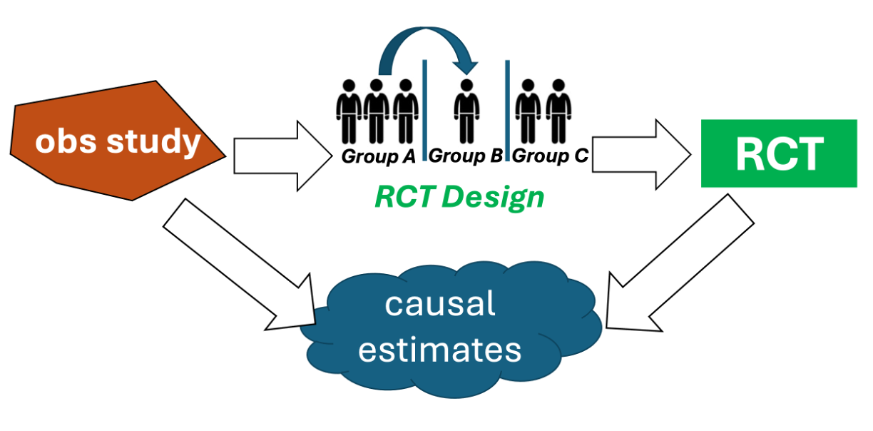
Figure 1: We use an observational study to construct our RCT design, and then the observational and RCT causal estimates are combined to increase efficiency.
To date, there has been limited attention to how these estimators might influence the design of a prospective experiment. If a researcher is designing a trial of a treatment, and already has some evidence about the treatment’s efficacy from observational studies, how might they alter choices about who to recruit and how to assign the treatment in the experiment? This is where the work we desribe below comes in: We provide a principled approach that works with data-combination estimators that are structured as Empirical Bayes ``shrinkage estimators” to determine ideal sample sizes for the targeted subgroups. We show the general flow of this idea in the figure above
What are we estimating?
In this work we are focused on estimating a vector of Conditional Average Treatment Effects (CATEs), \(\boldsymbol \tau = \left( \tau_1, \dots, \tau_K\right)\), one estimated impact for each subgroup. To be explicit, we are not primarily targeting a population-level ATE for the whole RCT or observational study. Each effect \(\tau_k\) corresponds to a subgroup of the data obtained by stratifying on the effect moderators. We seek to minimize the expectation of the squared error loss in estimating \(\boldsymbol \tau\) with an estimate \(\boldsymbol{\hat \tau}\), i.e.
\[\mathcal{R}\left( \boldsymbol \tau, \boldsymbol{\hat \tau} \right) = \mathbb{E}\left( \mathcal{L}\left( \boldsymbol \tau, \boldsymbol{\hat \tau} \right)\right) = \mathbb{E} \left( \sum_{k = 1}^K \left( \tau_k - \hat{\tau}_k\right)^2\right).\]
A simple example, given below, shows stratification on two variables: age and income. Both variables are measured in both datasets, and their values are discretized. The estimand in this case would be \(\boldsymbol \tau \in \mathbb{R}^{12}\).

Figure 2: Example stratification on two variables: age and income. The observational study has a different composition of strata than the RCT.
Choice of Estimator
A core component of our problem is that we know we are planning on using an estimator that borrows information across the observational and RCT datasets. We primarily work with a data-combination estimator from a prior paper of ours, Rosenman et al. (2020). The estimator is related to the famed James-Stein estimator. For \(\boldsymbol{\hat \tau_r}\) the vector of CATE estimates obtained from the RCT, \(\boldsymbol \Sigma_r\) its estimated variance, and \(\boldsymbol{\hat \tau_o}\) the vector of CATE estimates obtained from the observational study, the estimator is defined as \[ \boldsymbol \kappa_{1} = \boldsymbol{\hat \tau_r} - \left( \frac{\text{tr}(\boldsymbol \Sigma_r)}{(\boldsymbol{\hat \tau_o} - \boldsymbol{\hat \tau_r})^\mathsf{T} (\boldsymbol{\hat \tau_o} - \boldsymbol{\hat \tau_r})} \right) \left( \boldsymbol{\hat \tau_r} - \boldsymbol{\hat \tau_o} \right) \,.\] \(\boldsymbol \kappa_{1}\) shrinks each CATE estimate in \(\boldsymbol{\hat \tau_r}\) toward its counterpart in \(\boldsymbol{\hat \tau_o}\) by the same multiplicative factor in parentheses. This estimator is relatively intuitive to understand, and it often outperformed competitor estimators in simulations in Rosenman et al. (2020). So, as we design our experiments, we’ll plan on using \(\boldsymbol \kappa_{1}\). That said, the methods in our paper are somewhat general, and can be applied to a larger class of data-combination estimators.
In general, the logic of our approach is something like this: if the subgroup effects in the observational study are the same as in the RCT (something we can call transportability conditional on stratum), then the shrinking is a complete win. The more our observational study is biased, however, the more the point estimates of the RCT and the observational study will diverge beyond what we would expect given the uncertainty, and the less, therefore, we will shrink towards the observational result. This adaptability protects the integrety of the RCT and initial RCT subgroup estimates.
Proposed Design Methods
Givne the above, let’s design an experiment!
Specifically, consider the case where we have access to a completed observational study and are designing an RCT of the same treatment. The observational study and the prospective RCT will both be stratified on the same set of covariates. We plan to use \(\boldsymbol \kappa_1\) to combine the vector of CATE estimates \(\boldsymbol{\hat \tau_r}\) obtained from the eventual experiment, with \(\boldsymbol{\hat \tau_o}\), the vector of CATE estimates obtained from the observational study.
The problem at hand is how to best design the prospective RCT to reduce \(\mathcal{R}\left( \boldsymbol \tau, \boldsymbol{\hat \tau} \right)\), the expected squared error loss of \(\boldsymbol \kappa_1\). By “design,” we specifically mean how to choose the number of treated and control units per stratum, subject to a total sample size constraint of \(n_r\) for the whole experiment.
We are assisted by two powerful insights:
- The squared error loss of \(\boldsymbol \kappa_1\) can be written as a fraction of quadratic polynomials in Gaussian terms. Using recent results from Bao and Kan (2013), the expectation of such a fraction can be computed efficiently via numerical integration.
- Our objective function (the expected squared error loss) is thus a (complex) function of three inputs
- Treated and control sample sizes in each stratum: we optimize over these
- Variances of the potential outcomes in each stratum: we estimate these using the observational study
- Biases of \(\boldsymbol{\hat \tau_o}\) in each stratum due to unmeasured confounding: we can’t directly estimate these, but we consider various approaches to sidestep this challenge
With these results in hand, we propose three design heuristics to handle the bias term just above. The first is the simplest: ignore the shrinkage estimation completely, and determine sample sizes in the RCT using a Neyman Allocation (Splawa-Neyman, Dabrowska, and Speed (1990)), a well-known method for allocating sample sizes across strata based on the stratum-specific variances. Here, variances are estimated using the completed observational study (i.e. we assume our observational study is mostly correct).
In the second heuristic, we assume away the effects of unmeasured confounding, and minimize the expected squared error loss of \(\boldsymbol \kappa_1\) as though \(\boldsymbol{\hat \tau_o}\) were unbiased. At first blush, this might seem concerning. But the assumption of unbiasedness is used only for the phase of the experiment, not for inference. So if \(\boldsymbol{\hat \tau_o}\) is quite biased, this will just yield a suboptimal design, but it will not induce massive bias in our final causal estimates.
In the third heuristic, we constrain the magnitude of the bias in the observational study using a sensitivity model. Such models are widely used in causal inference to summarize the degree of unmeasured confounding. We make use of the popular marginal sensitivity model of Tan (2006), which summarizes the degree of confounding with a single parameter \(\Gamma \geq 1\). The analyst supplies a value of \(\Gamma\), and then solves for the best allocation under the worst-case bias in \(\boldsymbol{\hat \tau_o}\) possible given \(\Gamma\).
How much do we gain?
In partnership with the use of a shrinkage estimator like \(\boldsymbol \kappa_1\), the three heuristics allow us to build more efficient experiments that make use of prior observational data. To get a sense of the gains made, we simulate an observational study involving \(20,000\) units, in which the causal effect is biased due to failure to measure a key confounder. The simulations involve twelve strata, and we consider three different models for the treatment effect: one in which the impacts are constant across strata; one in which they grow linearly across strata; and one in which they grow quadratically across strata.
In the table below, we show results from simulations for an RCT with \(1,000\) units. We consider both the standard RCT-only causal estimator \(\boldsymbol{\hat \tau_r}\) and the shrinkage estimator \(\boldsymbol \kappa_1\), under each of the three treatment effect models. The columns correspond to different RCT designs: “Equal” is an equal allocation across strata; “Neyman” is a Neyman allocation; and “Naïve” is an allocation assuming no unmeasured confounding bias in \(\boldsymbol{\hat \tau_o}\). The subsequent four columns correspond to “robust” designs under the Tan sensitivity model, with different input values of the sensitivity parameter \(\Gamma\) (larger values mean more bias). This means that some cells correspond to experiments designed for \(\boldsymbol{\kappa_1}\) but where \(\boldsymbol{\hat \tau_r}\) was instead used, and vice versa.
| Estimator | Treatment Effect Model | Equal | Neyman | Naïve | Robust: \(\Gamma = 1.0\) | Robust: \(\Gamma = 1.1\) | Robust: \(\Gamma = 1.2\) | Robust: \(\Gamma = 1.5\) |
|---|---|---|---|---|---|---|---|---|
| \(\boldsymbol{\hat \tau_r}\) | constant | 100% | 91% | 92% | 91% | 94% | 94% | 98% |
| \(\boldsymbol \kappa_1\) | constant | 69% | 60% | 60% | 59% | 61% | 61% | 63% |
| \(\boldsymbol{\hat \tau_r}\) | linear | 100% | 93% | 93% | 93% | 95% | 97% | 99% |
| \(\boldsymbol \kappa_1\) | linear | 82% | 74% | 73% | 74% | 75% | 75% | 78% |
| \(\boldsymbol{\hat \tau_r}\) | quadratic | 100% | 88% | 90% | 91% | 92% | 92% | 97% |
| \(\boldsymbol \kappa_1\) | quadratic | 58% | 48% | 48% | 49% | 50% | 50% | 51% |
Within each design, the RCT data is sampled \(25,000\) times and CATE estimates are computed for each sample. In the table, the average squared error loss corresponding to each design is expressed as a percentage of the average loss of \(\boldsymbol{\hat \tau_r}\) using an equally allocated experiment, for each of the three treatment effect models. The minimum value in each row is denoted in bold. We see that \(\boldsymbol{\kappa_1}\) gives large reductions in expected loss, regardless of design. However, substantive gains are also achieved by using the proposed designs rather than an equal allocation. The Naïve allocation performs particularly well.
Our paper includes additional simulations and some more technical discussion, as well as an applied analysis using real data from the Women’s Health Initiative.
Discussion
We consider the challenge of designing a stratified experiment when we have access to an existing observational study measuring the same treatment. Using a shrinkage estimator such as \(\boldsymbol \kappa_1\), we intend to combine stratum CATE estimates from the prospective randomized trial and the completed observational study. Under this set-up, we propose three heuristics for the experimental design: Neyman allocation, naïve allocation assuming no unmeasured confounding in the observational study, and robust allocation under a sensitivity model for the confounding.
In a simulated scenario with a large observational database and a rare outcome, we observe significant risk reductions using shrinkage estimators, even with simple equal allocation designs. Additional gains are achieved by the use of our proposed designs.
This paper was a really fun collaboration, and employs ideas from two disparate areas of the statistics literature: Empirical Bayes methodology and experimental design. We are excited to share this work, which we hope will help practitioners to incorporate rich observational databases into improved experimental designs. Please reach out with any feedback or thoughts on future directions!