Recovering Effect Sizes from Dichotomous Variables Using Logistic Regression
by Josh Gilbert and Luke MiratrixThe Problem with Logistic Regression
In OLS regression with continuous outcomes, an omitted variable will not affect the estimation of an included variable if the omitted variable is uncorrelated with the included variable. This is not true of logistic regression: the point estimates in logistic regression change when variables are added to the model, even when the added variables are uncorrelated with the existing variables. In particular, the coefficients will be attenuated. This is because the residual variance of the logistic model is fixed at \(\pi^2/3\) (i.e., the variance of the standard logistic distribution) for model identification. Thus, when predictors are added to the model, as the residual variance cannot decrease, the coefficients on other variables will be driven upward.
This is a serious problem in interpreting the results of RCTs because even the independent treatment assignment indicator—by construction independent of everything—is not immune to this phenomenon. This means that the treatment impact we are estimating will change depending on what covariates we include in the model, limiting the utility of the analysis of binary outcomes such as “proficiency” that are common in educational research.
Note: This blog post has a lot of code (it has several simulations). The code has been extracted into the following file.
A Simple Simulation
To illustrate this phenomenon, we first write a simple simulation with a few parameters:
n: number of subjectsb1: treatment effect (logits)b2: continuous covariate effect (logits)k: cut point for a 1 vs. 0 dichotomized responsehet:TRUE/FALSEswitch for heteroskedasticity (whereTRUEdoubles the standard deviation in the treatment group)
make_data <- function(n = 500, b1 = 0.5, b2 = 1, k = 0, het = FALSE){

  tibble(
    id = 1:n,
    treat = rbinom(n, 1, 0.5),
    x2 = rnorm(n),
    y = b1*treat + b2*x2 + (1 + het*treat)*rlogis(n),
    prof = if_else(y > k, 1, 0)
  ) %>%
    return()

}
Below, I create a dataset tmp with 10000 observations and a b2 of 2.
tmp <- make_data(n = 1e5, b1 = 1, b2 = 2, het = 0)There is no correlation between treat and x2, as intended:
cor(tmp$treat, tmp$x2)## [1] 0.0002613427However, when I fit the logistic model without x2, the coefficient for treat is clearly attenuated, in contrast to the linear model on the continuous outcome y, which is not sensitive to the omission of x2.
m1 <- glm(prof ~ treat, tmp, family = binomial)
m2 <- glm(prof ~ treat + x2, tmp, family = binomial)
m3 <- lm(y ~ treat, tmp)
m4 <- lm(y ~ treat + x2, tmp)

tab_model(m1, m2, m3, m4,
          transform = NULL,
          show.dev = TRUE,
          show.r2 = FALSE,
          show.ci = FALSE,
p.style = "stars")| prof | prof | y | y | |
|---|---|---|---|---|
| Predictors | Log-Odds | Log-Odds | Estimates | Estimates |
| (Intercept) | 0.00 | 0.00 | 0.00 | -0.00 |
| treat | 0.62 *** | 1.01 *** | 1.00 *** | 1.00 *** |
| x2 | 2.01 *** | 2.01 *** | ||
| Observations | 100000 | 100000 | 100000 | 100000 |
| Deviance | 134020.905 | 89094.354 | 728742.629 | 326067.853 |
|
||||
The code below generalizes this process and repeats it with b2 varying from 0 to 4, with the other parameters fixed. For each b2 we create 20 replicates.
fit_mods <- function(data){

  m1 <- glm(prof ~ treat + x2, data, family = binomial) %>%
    tidy() %>%
    filter(term == "treat") %>%
    mutate(method = "Treat + X2")

  m2 <- glm(prof ~ treat, data, family = binomial) %>%
    tidy() %>%
    filter(term == "treat") %>%
    mutate(method = "Treat Only")

  bind_rows(m1, m2) %>%
    return()

}

analyze <- function(n = 500, b1 = 1, b2 = 1){

  tmp <- make_data(n = n,
                   b1 = b1,
                   b2 = b2)

  fit_mods(tmp) %>%
    mutate(n = n,
           b1 = b1,
           b2 = b2)

}

test_grid <- expand_grid(
  n = 1000,
  b1 = 1,
  b2 = c(0:4)
)

sims <- map(1:20, ~ pmap_dfr(test_grid, analyze, .id = "sim_id")) %>%
  bind_rows(.id = "rep_id")

sims <- sims %>%
  mutate(bias = estimate - b1)

ggplot(sims, aes(x = factor(b2), y = bias, color = method)) +
  geom_boxplot() +
  labs(x = "Beta 2",
       y = "Bias in Beta 1 (Logits)",
       color = "Estimation",
       title = "Omitted Variable Bias in Logistic Regression") +
  theme(legend.position = "bottom")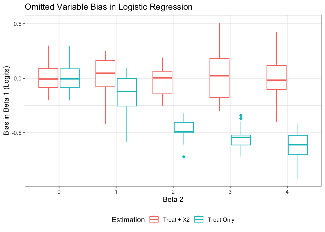
As expected, b1 is biased downward when x2 is omitted from the model, and the bias is worse the more strongly x2 is related to the outcome. Clearly, we must interpret logistic coefficients with caution, even in RCT contexts. This also means standard formulas for converting logits to effect sizes (such as dividing by \(\frac{\pi}{\sqrt{3}} = 1.81\)) can be incorrect1, or at least deceptive. Without good rules of thumb for how to think about an effect size in a logistic context, even the results of a well-designed RCT with a binary outcome can become difficult to interpret.
A Visual Illustration
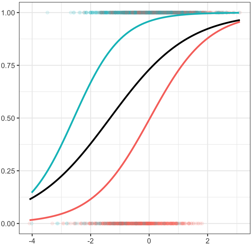
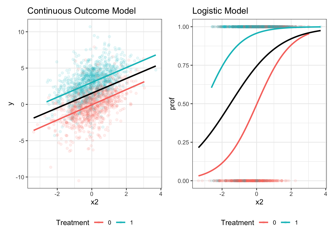
We can understand the phenomenon visually as well2. The continuous slope of y on x2 is unaffected by the exclusion of the treatment group indicator, but this is not true in the logistic model. In logistic regression, the cluster-specific or conditional slope of x2 differs from the marginal or population average slope, just as in multilevel logistic contexts.
A Potential Solution: Y-Standardization
One solution to the challenge interpreting logistic regression coefficients, proposed by Mood (2010) and others, is to estimate the standard deviation of the latent variable \(Y^*\) that could give rise to the observed responses and divide b1 by this value to “standardize” the estimates on the scale of \(Y^*\). The goal is to report our estimate in some sort of effect size unit with variation indexed by the latent continuous variable. This standardization would be:
\[ \begin{aligned} \beta_{ystd} &= \frac{\beta_{logit}}{SD(Y^*)} \\ SD(Y^*) &= \sqrt{\sigma^2_F + \pi^2/3} \\ \sigma^2_F &= var(\eta) \\ {\eta}&=\beta_0 + \beta_1 treat+ \beta_2 x_2 \end{aligned} \]
This method ideally puts all the logistic coefficients for treatment across different models on a single scale and allows cross-model comparisons. When the individual data are not available to calculate \(\sigma^2_F\), it can be calculated from descriptive statistics using the following formula: \[ \begin{aligned} \hat\sigma^2_F &= var(\hat\beta_0 + \hat\beta_1treat + \hat\beta_2 x_2) \\ &= \hat\beta_1^2 \times var(treat) + \hat\beta_2^2 \times var(x_2), \\ \end{aligned} \] using \(var(aX)=a^2var(X)\).
Thus, \(\sigma^2_F\) can be recovered from a table of regression coefficients and summary statistics, assuming the independence of the regressors.
However, it is not immediately clear what the y-standardized value means. Does it recover a type of standardized effect size for \(Y^*\)? The answer is a conditional yes: the y-standardized logistic coefficient is an unbiased estimator of a regression of a standardized variable on a treatment indicator in the continuous space under Homoskedasticity, as demonstrated in the simulation below, which compares the estimated regression coefficient on the standardized y outcome variable to the y-standardized logistic coefficient.
fit_mods <- function(data){

  # fit the model on the latent continuous variable
  m1 <- lm(y ~ treat + x2, data)

  # get the treatment coefficient
  b1 <- m1 %>%
    tidy() %>%
    filter(term == "treat") %>%
    select(estimate)

  # divide by SD(y)
  d <- b1[[1,1]]/sd(data$y)

  # fit the two logistic models
  m2 <- glm(prof ~ treat, data, family = binomial)
  m3 <- glm(prof ~ treat + x2, data, family = binomial)

  # get the latent vars from fitted values
  m2_var <- m2 %>% predict() %>% var() + 3.29
  m3_var <- m3 %>% predict() %>% var() + 3.29

  # get latent vars from coefs (to test that this method works)
  m2_var2 <- tidy(m2)[[2,2]]^2*var(data$treat) + 3.29
  m3_var2 <- tidy(m3)[[2,2]]^2*var(data$treat) + tidy(m3)[[3,2]]^2*var(data$x2) + 3.29

  # tidy the models and y-standardize the coefficients
  m2 <- m2 %>%
    tidy() %>%
    filter(term == "treat") %>%
    mutate(method = "T",
           estimate_std = estimate / sqrt(m2_var))

  m3 <- m3 %>%
    tidy() %>%
    filter(term == "treat") %>%
    mutate(method = "T + X",
           estimate_std = estimate / sqrt(m3_var))

  # combine and export
  bind_rows(m2, m3) %>%
    mutate(b1_y = b1$estimate,
           d = d,
           sigma2_f = c(m2_var, m3_var),
           sigma2_f_est = c(m2_var2, m3_var2)) %>%
    return()

}
Applying y-standardization method to our tmp data set yields a value fairly close to d for both logit models, even though the b1 differ substantially.
fit_mods(tmp) %>%
  select(method, estimate_std, d) %>%
kable(digits = 2)| method | estimate_std | d |
|---|---|---|
| T | 1.20 | 1.21 |
| T + X | 1.21 | 1.21 |
Below, I generalize this process to see how well y-standardization recovers the standardized effect size across a range of conditions.
analyze <- function(n = 500, b1 = 0.5, b2 = 1, k = 0, het = 0){

  make_data(n = n,
            b1 = b1,
            b2 = b2,
            k = k,
            het = het) %>%
    fit_mods() %>%
    mutate(n = n,
           b1 = b1,
           b2 = b2,
           k = k,
           het = het) %>%
    return()

}

test_grid <- expand_grid(
  n = c(100, 500, 1000),
  b1 = c(0, 0.2, 0.4),
  b2 = c(1, 2, 3),
  k = c(-1, 0, 1),
  het = c(0, 1)
)

# read in prior simulated data (will be overwritten later if needed)
sims <- NULL

if(RUN_SIMULATION == 1){

  plan(multisession, workers = 4)

  sims <- future_map(1:100, ~ pmap_dfr(test_grid, analyze, .id = "sim_id"),
                     .progress = TRUE,
                     .options = furrr_options(packages = "broom",
                                              seed = 2023)) %>%
  bind_rows(.id = "rep_id")

  sims <- sims %>%
    mutate(id = glue("{sim_id}-{rep_id}"),
         bias = d - estimate_std)

  write_csv(sims, "sims.csv")
} else {
    sims <- read_csv("sims.csv")
}
Results
Bias for \(\beta_1\)
b1 is unbiased on average across all conditions. However, when there is heteroskedasticity and the cut-point is not at 0, there are significant biases in the estimates, as shown in the table and figures below. A formal test of bias shows a significant interaction between het and k. That is, when the latent variable is homoskedastic, the cutpoint is irrelevant, but when the latent variable is heteroskedastic, a low cutpoint induces positive bias and a high cutpoint induces negative bias. Thus, the use of y-standardization to recover the standardized effect size in terms of the latent distribution depends on the assumption of homoskedasticity, or a cutpoint at the middle of the distribution, only the latter of which can be empirically verified with sample proportions near 50%.
sims %>%
  group_by(method) %>%
  summarise(bias = mean(bias)) %>%
kable(digits = 2)| method | bias |
|---|---|
| T | 0.01 |
| T + X | 0.00 |
sims %>%
  group_by(method, k, het) %>%
  summarise(bias = mean(bias)) %>%
kable(digits = 2)| method | k | het | bias |
|---|---|---|---|
| T | -1 | 0 | 0.01 |
| T | -1 | 1 | 0.13 |
| T | 0 | 0 | 0.01 |
| T | 0 | 1 | 0.01 |
| T | 1 | 0 | 0.00 |
| T | 1 | 1 | -0.11 |
| T + X | -1 | 0 | 0.00 |
| T + X | -1 | 1 | 0.13 |
| T + X | 0 | 0 | 0.00 |
| T + X | 0 | 1 | 0.01 |
| T + X | 1 | 0 | 0.00 |
| T + X | 1 | 1 | -0.12 |
sims %>%
  filter(n == 1000) |>
  ggplot(aes(x = d, y = estimate_std)) +
  geom_point(alpha = 0.1, size = 0.5) +
  geom_abline() +
  facet_grid(k~het, labeller = label_both) +
  labs(x = "Continuous ES",
       y = "Std B1 from Logit Model",
       caption = "Figure only plots N = 1000 for clarity")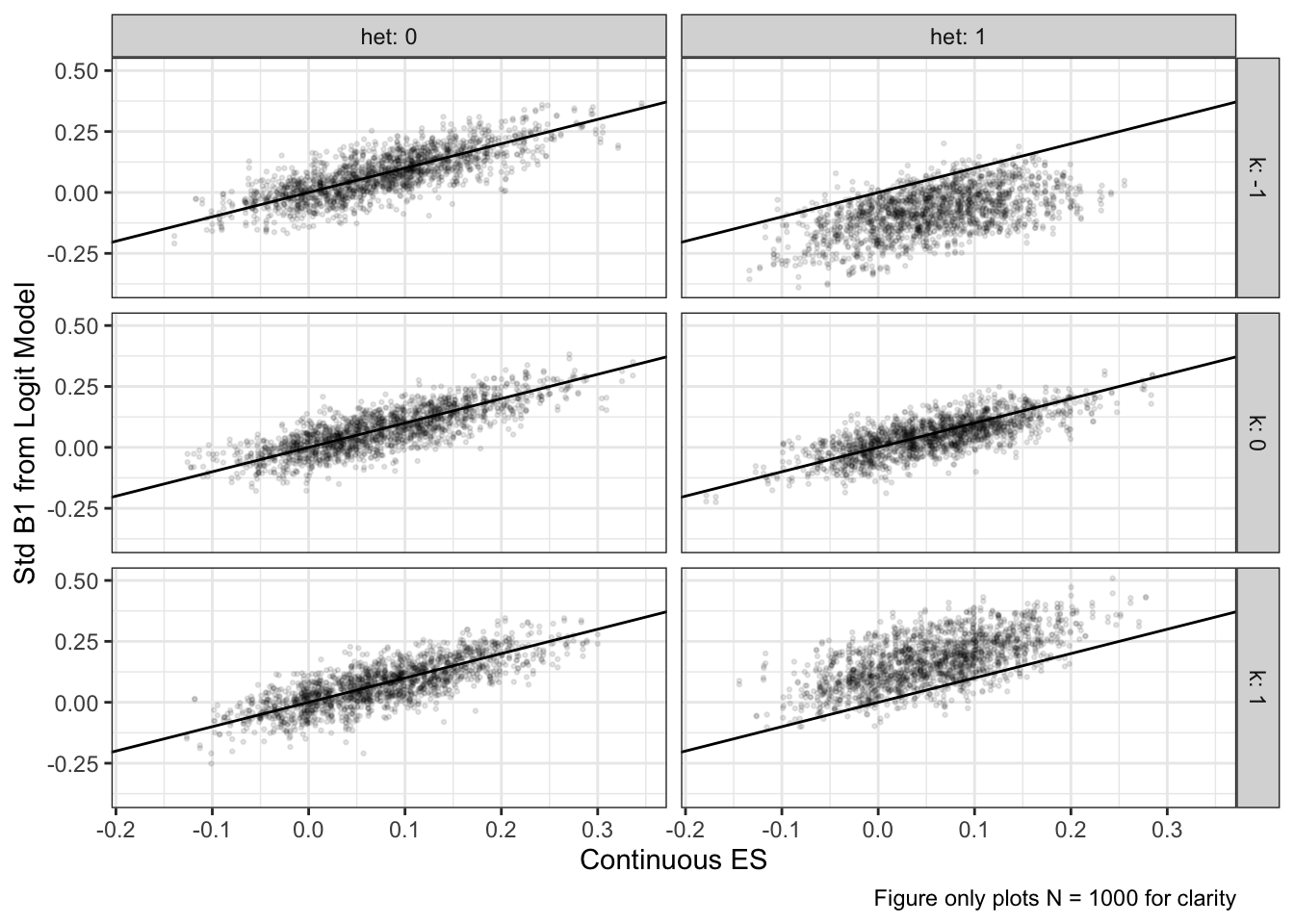
mlm <- lmer(bias ~ method + factor(n) + factor(b1) + factor(b2) + factor(k)*
       factor(het) + (1|id), sims)

tab_model(mlm,
          show.ci = FALSE,
          show.se = TRUE,
          p.style = "stars",
digits = 4)| bias | ||
|---|---|---|
| Predictors | Estimates | std. Error |
| (Intercept) | 0.0022 | 0.0030 |
| method [T + X] | -0.0044 *** | 0.0007 |
| n [500] | -0.0010 | 0.0021 |
| n [1000] | -0.0009 | 0.0021 |
| b1 [0.2] | 0.0058 ** | 0.0021 |
| b1 [0.4] | 0.0104 *** | 0.0021 |
| b2 [2] | 0.0014 | 0.0021 |
| b2 [3] | -0.0014 | 0.0021 |
| k [0] | -0.0014 | 0.0030 |
| k [1] | -0.0040 | 0.0030 |
| het [1] | 0.1263 *** | 0.0030 |
| k [0] × factor(het)1 | -0.1186 *** | 0.0043 |
| k [1] × factor(het)1 | -0.2404 *** | 0.0043 |
| Random Effects | ||
| σ2 | 0.00 | |
| τ00 id | 0.01 | |
| ICC | 0.75 | |
| N id | 16200 | |
| Observations | 32400 | |
| Marginal R2 / Conditional R2 | 0.262 / 0.812 | |
|
||
ggpredict(mlm, terms = c("het", "k")) |>
  ggplot(aes(x = factor(x), y = predicted, color = group)) +
  geom_point(position = position_dodge(width = 0.2)) +
  labs(y = "Bias",
       x = "Heteroskedasticity",
       color = "Cutpoint") +
  theme(legend.position = "bottom")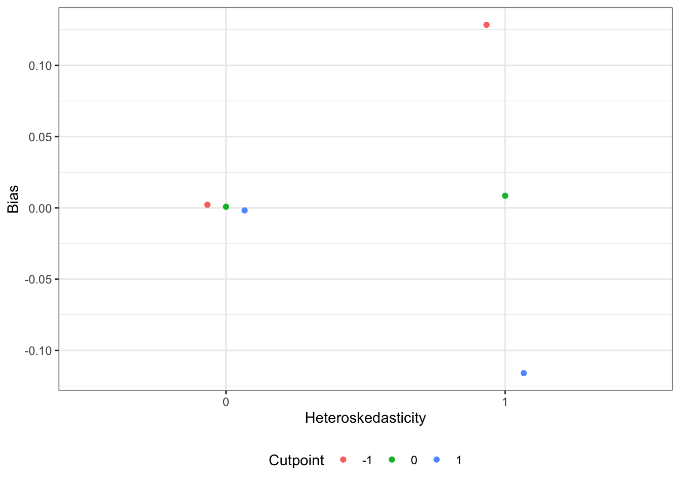
Estimation of \(\sigma^2_F\) from the Model and the Descriptive Statistics
Estimates of \(\sigma^2_F\) are nearly identical whether derived from the fitted values directly or from the parameter estimates and descriptive statistics, though this fact may be limited in its utility by the required assumption that the regressors are uncorrelated.
ggplot(sims, aes(x = log(sigma2_f, base = 10),
                 y = log(sigma2_f_est, base = 10))) +
  geom_point(alpha = 0.2) +
  geom_abline() +
  labs(x = "Sigma2 F estimated from Fitted Values (Log10)",
       y = "Sigma2 F estimated from Descriptive Statistics (Log10)")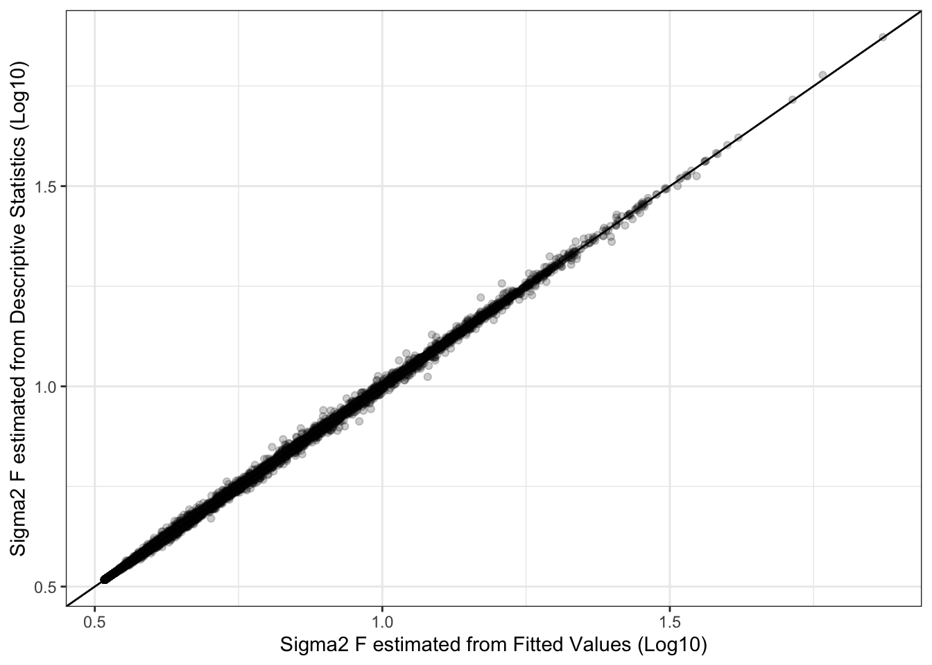
Application
NYC Charter Schools
I took publicly available aggregated data from NYC third graders in 2014. Each school reported the number of students who achieved “proficiency” based on state test scores. I used this information to create a student-level data set of the proficiency ratings and several school-level predictors. The (non-causal) “treatment” is whether the school is a charter school (charter). I ignore the clustering within schools here to focus on the point estimates.
# read in the data
nyc <- read_rds( file="nyc_school_sub.rds" )

# fit the logit models
nyc1 <- glm(prof ~ charter, nyc, family = binomial)

nyc2 <- glm(prof ~ charter + log2_enroll + percent_female + percent_poverty,
            nyc, family = binomial)
We see the point estimates are quite different between the models, but does this reflect the inflation of the coefficients or is it due to confounding between charter and the other variables? And how big is this logit difference on the actual test score scale?
tab_model(nyc1, nyc2,
          transform = NULL,
          show.ci = FALSE,
          show.r2 = FALSE,
p.style = "stars")| prof | prof | |
|---|---|---|
| Predictors | Log-Odds | Log-Odds |
| (Intercept) | -0.81 *** | -0.57 *** |
| charter | 0.27 *** | 0.54 *** |
| log2 enroll | 0.14 *** | |
| percent female | 0.01 *** | |
| percent poverty | -0.03 *** | |
| Observations | 74420 | 74420 |
|
||
The code below estimates the latent SDs allows us to standardize the estimates and interpret them on the continuous test score scale, and we see that the mean difference increases from 0.15SDs to 0.28SDs when the covariates are added to the model (assuming homoskedasticity). This suggests that the covariates are masking the strength of the unconfounded association.
sd1 <- ((predict(nyc1)) %>% var() + 3.29) %>% sqrt()
sd2 <- ((predict(nyc2)) %>% var() + 3.29) %>% sqrt()

tidy(nyc1)[[2,2]]/sd1
## [1] 0.1470456tidy(nyc2)[[2,2]]/sd2## [1] 0.2784896References
Inspired by this blog post: http://jakewestfall.org/blog/index.php/2018/03/12/logistic-regression-is-not-fucked/↩︎