Contextualizing point estimates and p-Values

Once an analysis is in, we need to think carefully about how to talk about our results. Statistics is about inference, about capturing the uncertainty in our findings given limitations of our data and estimation error. We want the reader to quickly assess how seriously to take an estimated difference, and we want to present our results in way that is fair (are not overly pessimistic about what the data mean) while not being misleading (making differences seem less likely to be a result of random chance than they are).

These concerns is what drives the use of confidence intervals and \(p\)-values. And this is where we start to see people get agitated: in particular, there has been a lot of furor over \(p\)-values of late. Are they useful? What should we do with them? The American Statistican recently had a series of articles on \(p\)-values where various people proposed several ideas and alteratives. A few jumped out at me as being of particular interest. For me, the core concern is what makes for an effective communication strategy.

One proposed idea is to take a confidence interval and interpret the upper and lower range of the confidence interval in terms of practical significance. For example, say we had teacher PD program that was found to increase student test scores by \(0.22\sigma\) with \(p \approx 0.037\) (i.e., the average of the treatment students were \(0.22\sigma\) higher than the control students, in effect size units, and this increase was statistically significant).

To contextualize these findings, we would want to first have a confidence interval for these findings. In our case the 95% confidence interval would be \(0.01\sigma - 0.43\sigma\). If we interpret the endpoints of this interval we would conclude that our program could potentially have almost no impact on student outcome, or could have an impact of almost a half standard deviation. This range is not very meaningful, or useful. It does communicate that, when significantly pressed, all we can say is the program didn’t cause harm, and could have done a great deal.

One issue with this approach is that we are intepreting two possible circumstances, but these circumstances are the most extreme. Instead, we could interpret a more moderate range. I propose taking the 80% confidence interval (here this means an interval of \(0.08 - 0.36\)). Now we would say that we found substantial evidence that our program was beneficial. On the poorer end, we achieved a modest gain in student outcomes, and on the optimistic end we could have achieved impacts of 3 or 4 tenths of a standard deviation, which would be noteworthy.

Of course, if we could express these findings in something other than effect size units, such as fractions of a year of growth, or similar, then all the better.

Taking this one step further, if we reflect on what a standard error means we realize that it is our best guess as to how far off our estimate is from the truth. Flipping this on its head, we are saying that the truth is about 1 SE away from our point estimate. Then, instead of interpreting our point estimate, we should mark the two contexts that are 1 SE away. In other words, we should consider a 68% confidence interval (under a normal approximation). In our running example, this would be \(0.11\sigma - 0.32\sigma\), not substantially different from our 80% case.

The bottom line is that the usual levels of confidence (e.g., 95%) give intervals that hold some fairly extreme (and unlikely) estimates of the truth. Of the range of outcomes in a 95% interval, 35% of it lies outside the 80% interval (i.e, 95% intervals are about 50% longer than 80% intervals). In other words, the additional 15 percentage points of “probability mass” gained by moving to a 95% interval from an 80% interval entails a large expansion of range. See figure, below, that shows how confidence and interval length are related. Increasing the level of certainty for a confidence interval is increasingly expensive in terms of its length.

Take aways. When interpreting results, to take into account estimation error, we should interpret two different scenarios: a plausible optimistic scenario, and a plausible pessimistic scenario. This can be done with a 68% or 80% interval (they will tend to be similar, with the 80% having more extreme scenarios, and the 68% capturing two reasonable “best guesses” of our likely being off the mark by a standard error or so.

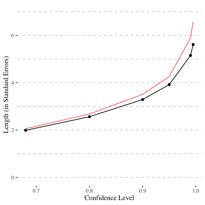
Remark. In this figure, the red line denotes a confidence interval built from a \(t_{15}\) distribution, which is a bit more extreme.

Comments:

References

Wasserstein, R. L., Schirm, A. L., & Lazar, N. A. (2019). Moving to a World Beyond \(p < 0.05\). The American Statistician, 73, 1–19. http://doi.org/10.1080/00031305.2019.1583913